[+ Font] :: [- Font] :: Printable

Natural Gas: A Long Modern Survey (Part 1)

Professor Ferdinand E. Banks
November 13, 2007
ferdinand.banks@telia.com
The University of Uppsala, Uppsala Sweden
The School of Engineering, Asian Institute of Technology, Bangkok Thailand

Part 2



ABSTRACT: By "modern" survey I mean a survey that presents items and issues with which readers should be familiar, but for one reason or another are often unaware. This is important because, according to Daniel Yergin of Cambridge Energy Research, the biggest challenge facing the U.S. energy sector today is ensuring the availability of sufficient gas supplies. I can add that what we should avoid at all costs is an unexpected peaking of e.g. global oil and gas production, which could not only lead to economic and political chaos, but even to wars as major consuming countries elect to employ their military assets to obtain a satisfactory share of remaining resources. I attempt in this paper to correct and update the discussions in my book on natural gas (1987), as well extend the chapters on gas in my two energy economics textbooks (2000, 2007); and I also hope to provide readers who absorb a large part of the exposition with a 'competitive advantage' in their interaction with teachers, students, colleagues and/or adversaries. Unfortunately the inclusion of some mathematics in this contribution could not be avoided for pedagogical reasons, although some of it can be easily bypassed.

Keywords: Reserve-production ratio, Russian gas, gas deregulation, gas pipelines

1. INTRODUCTION
In many respects, natural gas is an ideal fuel. Its environmental qualities (in terms of its emissions of 'greenhouse' gases) are helping to make it the most demanded of the fossil fuels (i.e. gas, oil and coal), and there is a great deal of it in the crust of the earth - though not as much as many observers believe. As pointed out by Ken Chew (2003), the amount of gas resources discovered annually peaked in the beginning of the l970s, and the number of discoveries early in the l980s. (This lends weight to a contention by Julian Darley (2004) that gas production could 'plateau' before 2025.) Natural gas is found in appreciable quantities in very many countries, and Russia has the world's largest reserves and is the biggest producer. The United States (U.S.) is the largest consumer, and although it has about 3% of world reserves, Europe (excluding Russia and Eurasia) consumes roughly 20% of global output. Considerable gas has attained the status of 'stranded gas', which means gas that has been discovered but is not economically viable for physical or economic reasons: for instance, it is too far from main pipeline routes, or localities where gas consumption is high, to make its exploitation attractive.

Since l980 natural gas has exhibited the fastest consumption growth of all fossil fuels - averaging between 2.5 percent per year (= 2.5%/y) and 3%/y. Only primary electricity exceeded this figure over the same period, averaging almost 4%/y. (Primary energy is energy obtained from the direct burning of coal, gas, oil, etc, as well as electricity having a hydro or nuclear origin. Electricity obtained from e.g. a gas turbine is a secondary energy resource.) The average energy content of natural gas varies from a low of 845 British Thermal Units per cubic foot (845 Btu/cf = 845 Btu/ft3) in Holland to 1300 Btu/ft3 in Ecuador. In Russia it averages 1009 Btu/ft3 and in the United States (U.S.) 1025 Btu/ft3. In this article, as in my textbooks, I follow the usual practice of rounding these numbers to 1000 Btu/ft3: this is a number that students of energy economics should always have at their finger tips, and it is more important than the equivalent amount in Btu/cubic meter (= 28.6 Btu/m3). You should also note the difference between energy - which above is in Btu - and power, which is relevant later in the discussion of compressors for pipelines, where it is measured in horsepower.

North America (including Mexico) has about 5.1% of world gas reserves, with the United States (U.S,) holding the largest part. South America has about 4.8%, with Venezuela being the largest possessor. Western Europe about 3%, and surprisingly The Netherlands has more than the UK (48 trillion ft3 (= 48 Tft3 ) versus 17 Tft3 , but much less than Norway (102 Tft3). However even so, because of its location and storage facilities, The Netherlands is regarded as the swing producer for the Western European gas market, which implies that if there were a sudden decline in the physical availability of gas , that country could (and ostensibly would) fill the gap - which may or may not be true. Saudi Arabia has been pictured as playing this role for the world oil market, however with the rapid increase in the global consumption of oil, it may not be able to perform this function much longer - even if it wanted to. Global reserves are approximately 6405 Tft3, and production about 2865 billion cubic meters (= 2865 bcm).

Eurasia (= Russia, Ukraine and Central Asia) has about 36% of global reserves, with Russia, the gas superpower, in possession of 85% of these. An important observation that can be offered here is that the extensive deregulation of gas that is scheduled to take place in the European Union (EU) may result in greatly increasing the market power - i.e. the monopoly or oligopoly power - of Russian gas exporters. The sponsors of this deregulation are apparently unfamiliar with the economic logic supporting this uncomfortable prospect, and so it might be suitable to point out that collusion on the buying side of the wholesale gas market (which is where large buyers obtain gas from external producers), together with continued regulation on the selling side of the retail market (which involves final consumers), could optimize the welfare of Western European firms and households who are becoming increasingly dependent on foreign resources This is because the bargaining power of the aggregate of large buyers might be increased. Decision makers in the gas importing countries should attempt to understand this situation, because important forecasting establishments claim that with global gas demand scheduled to almost double by 2025, gas prices could escalate.

The Middle East has about 36% of global reserves, with Iran possessing almost 50% of this amount, but Qatar is the most important exporter of gas in this region, and has become the leading global supplier of liquefied natural gas (LNG). Africa has 7%, with most of it in Nigeria and Algeria; and there is slightly more than 8% in Asia and Oceania, with Australia, Indonesia and Malaysia being the main players. As is the case with oil, China is going to require an enormous amount of gas, and perhaps more than is or will become available from its present key suppliers, Australia and Indonesia. The U.S. remains the world's largest gas market, but Japan is the largest importer of LNG, and enjoys the considerable advantages that come with being able to exercise market power - in this case monopsony - when confronted by its present suppliers.

Altogether there are approximately 6405 trillion cubic feet (or 224 trillion cubic meters) of proved reserves in the world, but appearances sometimes deceive. The United States cannot be regarded as particularly favoured any longer where gas is concerned, given the forecasts of its huge future consumption. It also appears that the U.S. does not produce much more gas today than was produced 30 years ago. In addition, the reliance of that country on suppliers outside North America (and Mexico) steadily increases. These suppliers include distant countries that at the present time are able to ship only limited quantities of liquefied natural gas (LNG) to North America, and in addition a shortage of existing and planned terminals for receiving more gas is evident. Another country that might be moving into an unfavourable gas position is the United Kingdom (UK), where oil production recently peaked, and domestic gas reserves will soon be unable to support expected consumption. There is an important lesson here. As in California, a very large inventory of gas-based facilities came into existence because of technical improvements in gas burning equipment and low gas prices; while later (for a while) it appeared that it was more economical to pay higher prices for gas than to invest in alternative sources of energy. Thus we have another predicament in which, in the presence of uncertainty, we see the advantages of sometimes having a highly diverse portfolio of assets - e.g. gas, coal, nuclear, renewables - instead of "falling in love" with a single energy medium, as pointed out once in Forbes.

One purpose of this paper is to clarify important issues that have not been adequately treated in much of the literature. For example, theories about the abundance of natural gas are often based on the observed size of the existing reserve-production ratio (= Q/q ratio), where Q is units of reserves, and q is output per year. For gas, this ratio was about 63 (years) at the beginning of 2007, implying that even if no more gas is discovered, current production can be maintained for more than 6 decades. (Similar thoughts prevail for oil, whose global Q/q ratio is close to 40.) Most geologists - though not most economists - understand the futility of this approach, because prima facie it suggests that current production could be maintained for Q/q years, and then terminated almost immediately. It also fails to stress the possibility of a comparatively early peaking of output, as well as the economic logic underlying this phenomenon for both gas and oil.

When we examine production profiles in major oil or gas region in e.g. the United States, what we see is a rising output (or build-up for oil and gas) that eventually peaks, perhaps forms a plateau, and eventually begins to decline, even though there may still be a huge amount of the resource in the ground. As shown in Figure 1, there is a decline with or without additional investment designed to extend the life of the structure. The reason (and perhaps the only reason) is that on the basis of reserves that have been identified in a particular deposit of field, it is uneconomical to attempt to prolong the plateau indefinitely!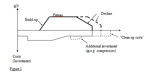



If the explanation for this configuration turns on economics and not geology, an explanation is due. Let's start with the following equation, which has to do with the maximization of discounted profits (= discounted Revenue minus Cost) over N periods.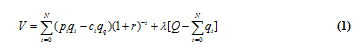



In the first parenthesis we have expected profits in period ‘t’, or expected revenue (R_t = p_tq_t) minus expected cost (Ct =c_tq_t), while in the third parenthesis we have the predicted amount of the resource (e.g. gas), Q, that will be distributed in an optimal manner over N periods (q₁ + q₂ +…..+ q_N = Q). The second parenthesis, (1+r)^-t, merely discounts the profit in period ‘t’: profits in distant periods have less value than those of e.g. today. It might also be useful to know that S (R_t – C_t)/(1+r)t is sometimes called the capital value of future receipts: it is the current price of the rights to a stream of future – or expected future – receipts. In conventional presentations N is taken as given, and ‘c’ is usually regarded as a constant that is equal to both average and marginal cost for the N periods. The implicit assumption here is that prices and costs, as well as the amount of the resource, are correctly forecast at the beginning of the current period. λ is a Lagrangian multiplier, and gives us the scarcity value of the resource: e.g. it is zero if R exceeds the amount of the resource expected to be extracted during the N periods (because then the resource is not scarce). In these circumstances, if we differentiate V with respect to the values of q, and manipulate slightly, we obtain the famous Hotelling (1931) expression ?p/p = r, where p here is defined as the 'net' price - or price minus the marginal cost - and this net price increases at the rate r. In terms of the real world, where the ex-post (i.e. after the fact) production curves of gas take on the appearance of the curve in Figure 1 (or even a distinct 'bell' or 'normal' appearance), this is a nonsense result! In order to obtain something approximating realistic production curves, it is necessary to assume that 'c' can increase as time passes and the deposit is gradually exhausted. This is because the most important variable for an individual deposit is NOT 'r' - which your favourite economics teacher might told you - but deposit pressure and its significance for the cost of extraction. As gas is removed and deposit pressure falls, it may be necessary to introduce additional wells or pressure augmenting activities in order to maintain output. If you saw the film 'Five Easy Pieces', the good Jack Nicholson was apparently occupied with work that was intended to compensate for the decline of an oil deposit. Had it been gas instead of oil, the same observation is valid.

For students of energy economics, the basic issue here can be shown with a simple equation. In my lectures I sometimes use C = αx /(β - x ), where C is the cost (in some monetary unit) of removing x percent of a deposit, and α and β are constants. If for example β was equal to 100, then C approaches infinity when the deposit approaches exhaustion. At this point readers might substitute a few values of x in the equation in order to see what happens to C, however it is just as simple to look at a couple of derivatives: dC/dx = αβ/ (β - x)² and d²/dx² = 2αβ/ (β- x)³. Both are positive, and so not only does cost increase as more of the deposit is removed, but this increase 'accelerates'.

In considering the present topic, it is also essential to be aware of something called the 'natural decline rate', which involves the 'deterioration' of a deposit due to previous production, but like deposit pressure does not explicitly enter into the above expression. Before saying something about the decline rate however, it should be noted that the same kind of production pattern illustrated above will likely be duplicated on a global scale, and unfortunately sooner than many readers of this paper expect. On the basis of present supply-demand trends, it is possible, though not certain, that in 20-25 years the output of gas will peak, and after a short or long plateau, begin to decrease. It has been suggested that the bad news about gas will not take a minimum of 20 years to appear, as the former Chairman of the Federal Reserve System Alan Greenspan flatly stated in his testimony before the Committee on Energy and Commerce of the United States House of Representatives in June, 2003. On that occasion the Chairman was not thinking of in terms of depletion but of price, and he had good reason for his concern.

The least complicated equation for discussing this matter is probably the one given directly below, where we are discussing a case that in economic theory is called 'depreciation by evaporation', and in which an asset is subject to a constant force of mortality 'Ө'. The relevant equation takes on the following appearance.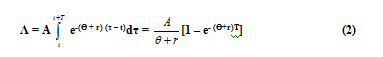


In this expression A is the amount of the asset, and r is a discount rate. It would be a simple matter to make 'Ө' a function of the 'deterioration' of the asset.

Equations (1) and (2) could possibly serve as a starting point for a comprehensive exposition if some readers were not allergic to integrals, but in any case the important thing is an interpretation of (2). What this expression says is that the presence of a natural decline reduces the value (Λ) of the deposit. More important, the mere fact of depreciation means that output can only be maintained as a result of investment, and as alluded to earlier, in the long run investment might become too expensive. This theme can be approached without calculus, but even so requires too extensive a discussion of the economics for this rudimentary presentation. It might be useful to suggest though that an implicit investment function with investment designated as I and revenues R (=pq) obtained from investment might serve as the starting point for this exposition. With reference to e.g. Figure 1, that function would take on the appearance ?(I₁, I₁,…,I_T; R₂, R₃…,R_T+1) for periods '1' to e.g. 'T+1'.

Next we should carefully note that 1000 cubic feet (or 28.6 cubic meters) of gas has an average heating value of approximately 1,000,000 British Thermal Units (= 1 mBtu). (The exact figure, as noted earlier, may be as much as ten percent higher or lower.) One barrel of oil has an average heating value of 5,800,000 Btu. Only a few years ago OPEC still expressed its intentions to keep the world oil price between $22 and $28 per barrel (=$/b) if possible, and so we can immediately calculate that this corresponds to a gas price of $3.8/mBtu to $4.8/mBtu, where 'm' signifies million. Something of interest here is that long before the oil price began its present ascent, there was an occasion when the gas price in the US spiked to $10/mBtu (= $58/b in oil terms), and a similar phenomenon was observed in Mexico. Numbers like these concentrated more than a few minds at the upper political levels in the energy intensive countries, but worse may be in store, since the OPEC countries may have come to the conclusion that $70/b is the lowest price at which they should sell oil. This corresponds to an 'oil equivalent' price for gas of $12/mBty. In the third section of this paper I examine price formation in the natural gas market, and touch on this subject once more.

It seems likely that just about everybody interested in energy has heard gas referred to as the 'fuel of the future'. In fact I used this expression several times in my first energy economics textbook (2000). But although I emphasized gas' relatively favourable environmental properties, it should not be forgotten that gas also emits a sizable quantity of carbon dioxide (CO₂), and its high methane content makes it less attractive than often portrayed to TV audiences.

Readers should also never lose sight of the fact that, despite the growing important of gas, in terms of physical fundamentals oil is still the most valuable energy resource. For instance, as energy resources must be moved over longer and longer distances from large suppliers to large buyers, gas' relatively inferiority to oil increases. Whether by pipeline or tanker, the unit transport costs of oil are lower than those of gas. If we consider a given volume of pipe, oil contains (on the average) 15 times as much energy as gas, which immediately reflects - negatively - on pipeline investment costs for gas. Furthermore, when considering intercontinental trade, transporting gas by ship over all except very long distances is more expensive than by pipeline, while transporting oil by tanker over the same distances is less expensive than by pipeline. This is one of the reasons why, quantitatively, the kind of global competitive market that various observers hope or expect will come into existence after enormously expensive LNG investments are carried out, may prove to be disappointing.

As with oil, there are plenty of energy professionals ready to claim that technological advances will ensure that we will always be able to obtain the gas and other energy resources we need at prices that we can afford. The technology booster club is now turning its attention toward innovations that might make it possible to exploit vast deposits of crystallized natural gas suspended in Arctic ice, or buried just below the ocean floor, and which are known as methane hydrate. Optimists even claim that it is now possible to obtain controlled volumes of methane from a hydrate-rich area in North Canada, and apparently some or all of this hydrate-based gas has been officially classified a viable energy reserve.

Similar extravagant claims are being advanced about a big slice of the oil in Alberta that is extracted from tar sands, and which in theory is capable of making Canada an oil producer of the Gulf format. In truth only the richest of these resources are worth exploiting until oil and gas prices escalate even more, and then the laws of thermodynamics may stand in the way of making energy dreams come true. The problem seems to be that it may take more energy to exploit these 'unconventional' resources than they contain, and much of this energy might have to come from expensive natural gas - although I have occasionally argued in my lectures that under certain circumstances this trade-off is acceptable. If, for example, an inexpensive energy source could be transformed into expensive synthetic oil, then thermodynamic considerations may not be so important in the short run. According to official forecasts, it will not be before 2020 that Canadian tar sands can provide a modest 4mb/d of oil.

2. SOME ASPECTS OF ECONOMIC THEORY AND GAS PIPELINES
There is always a problem in a presentation of this nature concerning the choice of topics to be reviewed. In my first energy economics textbook I had a fairly long discussion of gas pipelines, while in the latest textbook - which is designed to be an introductory textbook - this topic was only treated en passant. As I found out in my lectures in Bangkok, some students wanted more attention paid to gas pipelines, and so what I shall do now is to extend the discussion in my earlier textbook. Readers who want a very thorough exposition of the economics of gas pipelines should examine the work of the late Hollis Chenery (1949, 1952). Let me emphasize though that what is taking place below is to obtain a production relationship that can provide optimal values of the inputs with a given amount of gas to be transported a certain distance.

Perhaps the best way to begin the exposition is with a diagram showing some of the elements in a typical pipeline. This is presented below.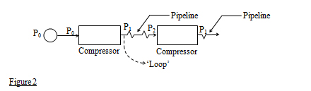



As we should note from this diagram, a gas pipeline is a fairly complicated structure. There will be considerable algebra in this section, but before we come to that it seems appropriate to peruse certain important concepts. To begin, readers should understand the expression sunk costs. Sunk costs are expenditures that, once made, cannot be recovered: they are associated with decisions that cannot be reversed later. A pipeline that costs billions of dollars can be chopped up and sold to scrap dealers for thousands or a few millions, but conceptually it seems appropriate to regard the main gas transmission lines as sunk investments. (On the other hand, a fixed cost is a cost that is fixed in the short run. A 'crack house' can be renovated and turned into a luxurious town house - at least in theory.) The most important costs associated with a gas pipeline are planning and design, acquisition and clearing of right-of-way, construction and material costs (e.g. labor costs, the cost of pipes and compressors, etc), the cost of monitoring the pipeline and performing maintenance, and energy to power the compressors (which are analogous to pumps in an oil pipeline, in that they transfer mechanical energy from e.g. a motor to the gas that is to be transported).

The expected life of a gas pipeline can exceed 30 years, and the investment can be extremely large. Russia has promised to build two pipelines to China, and their cost is estimated at 10 billion dollars. Strictly speaking, a pipeline cost should be regarded as sunk, but for pedagogical reasons no distinction will be made between sunk and fixed costs, since in almost all economics textbooks the word "sunk" seldom appears in the chapters on production theory. On the other hand, the expression 'increasing returns to scale' is often used in discussions of the sort that will be carried out here, and so I want to present a simple example which applies to both oil and gas pipelines.

In designing a gas pipeline, engineers might think in terms of varying the pipeline diameter and the number and size of compressors, as well as things like the amount of maintenance that will be required. Increasing the size (and energy output) of a compressor, without changing the diameter, raises the speed at which the commodity goes through the line, and thus increases the 'throughput' of a given size pipe. Similarly, increasing the diameter of a line with the compressor size constant, might also raise throughput, since there is less resistance to flow (per cubic feet of gas) in a larger pipeline. A fundamental issue here is how much of the commodity is in contact with the inside of the pipe, and not just the total volume of throughput.

By way of extending this simple observation, remember that the volume of a pipe of length L, with radius r, is πr2L. (For convenience, take L = 1 foot or 1 meter). The inside surface area of the same pipe is 2πrL. If the radius is doubled the surface area is also doubled, but the volume of the interior of the pipe is increased by a factor of four! Furthermore, a small amount of algebra informs us that there is less surface area per unit of volume for larger diameter pipes than for pipes with a smaller diameter, and as a result there is less frictional resistance per unit of throughput for a larger than for a smaller pipe. Then why not increase the radius of the pipe indefinitely in order to exploit the returns to scale being described? The answer - as you discovered in Economics 101 - is that at some point it is less expensive to raise throughput by a marginal addition to compression than by increasing the pipe diameter. I can add that just as (ceteris paribus) we have returns to scale in the pipe, we might also have returns to scale in compression, at least up to a certain point. You can think about this prospect in terms of the 'soup-bowl' diagrams that you enjoyed sketching in your first course in economics, and which applied to many kinds of equipment.

It has been suggested that if a pipeline manager is in position to raise (transmission) prices after gas producers have made their drilling and development investments, it will cause risk averse gas producers to limit the size of their investments in order to avoid being unpleasantly surprised by an increased price of transmission. This reasoning also works in the other direction. If gas producers have several pipelines through which to transmit their output, it could place pipeline managers in a dilemma in that they would always face the threat of gas producers transferring their affections to another carrier. On the national level this suggests that an optimum arrangement might call for a single owner for gas deposits and pipelines. A similar provision 'might' be possible internationally, but this is less likely. Instead, the optimal solution probably turns out to be complicated but necessary long term contracts. Under no circumstances does it mean an enthusiastic resort to short term arrangements that the EU Energy Directorate is trying to promote except, possibly, in very special cases.

What is being said here is that firms to not want to find themselves in possession of a large amount of worthless capital equipment - e.g. equipment that becomes worthless because the demand for pipeline capacity or gas suddenly and drastically collapses. The algebra of this situation will be avoided because it involves some probability theory, however if a firm is risk averse and wants to avoid the financial dangers associated with excessive investment in fixed or sunk capital, then long term commitments make a great deal of economic sense. It is difficult for me to see how a rational person could come to any other conclusion.

In order to carry on an elementary but meaningful discussion of the economics of gas pipelines, it is useful to put the production relationship into the form of the kind of production function that you encountered in your introductory economics courses, where output is a recognizable function of inputs. In the present discussion there is no problem with output (i.e. gas), although inputs (pipe and compressor size/capacity) might require some thought. But before beginning this exercise, I want to present a simplified version of an article written by R.E. Hodges (1985), in which there were three engineering relationships having to do with natural gas that were developed by the American Petroleum Institute. Some readers might prefer this departure to systematically formulating an optimization problem of the kind presented in intermediate economic theory.

If we take the output of the pipeline given, and equal to q*, then Hodge's first equation was for the gas velocity in a pipeline at the output of a compressor, and this is taken as a function of pipe diameter (D), and pressure at the outlet (p₁). Implicitly this equation is V = V(D,p₁), with δV/δD < 0 and δV/δp₁ > 0: with a given exit pressure for a compressor, velocity decreases as the diameter increases; and with a given diameter velocity increases as exit pressure increases. If the equation for V was written in explicit form, it would contain a number of thermodynamical constants/parameters, and in the last equation below the allowable stress of the metal used in the pipeline is also included.

The next equation is for what Hodges calls a friction factor, and this can be written F = F(V,D). A high gas velocity and a large diameter mitigate pipe friction, and so we have δF/δD < 0 and δF/δV < 0; however we can get rid of the V by substituting from the first equation, which gives us F = F(p₁,D), which is very convenient. Finally, the (recommended) pressure decline in a (given) length of pipe (L) between compressor stations, and with given output q*, depends on p1, D, and F, (as well as the aforementioned thermodynamical constants). This can be written ?p = p₁ - p₂ = g(p₁, D, F), where length and output enter the equation as parameters. Since F is a function of p₁ and D however, we can again make a substitution and obtain Δp = g(p₁, D), or p₁ = p₂ + g(p₁, D). In the light of the discussion that will follow, p1 can be considered a proxy for compression - i.e. the 'size' or rated capacity of the compressor (in horsepower). If we have the cost of pipe and the cost of compression, then by juggling these relations - probably with the help of a computer - we can obtain the optimal values of D and p₁, where optimal in this case means values that give us the lowest total cost.

In a similar vein, Chenery began his analysis by writing two equations for the system, with the first being an engineering relationship governing the flow of gas, or q = Kf(D, p₁, p₂). K is a constant covering a number of thermodynamical factors (such as temperatures and specific gravity of the gas), D is the diameter of the pipe, p1 is the outlet pressure from a compressor, and p2 the inlet pressure. These pressures are shown in Figure 2, and it might be useful here to give an example of the equation used by Chenery, which is q = KD8/3(p12 - p22)1/2 = KD8/3p₁[1 - (p₂/p₁)2]1/2. . A prominent shortcoming in this equation is that the distance between compressors (L) is not present, and this deficiency is not entirely ameliorated by Chenery's decision to standardize the distance to 100 miles. The thing to understand though is that Chenery was dealing in economics and not engineering, which provided him (and me) with a certain indulgence.

Considering the discussion of pipelines from Russia to Western Europe that took place at the Stockholm School of Economics recently, it became clear that the distance between compressors is an important variable, and in line with the work of Paulette (1968), it might be better to write the implicit relationship above as q = Kf(D, p₁ , p₂ ,L). Then, with q 'given', and some sophisticated (and perhaps computer aided) assumptions about the two pressures, it might be possible to solve for the optimal distance between compressors. However I am not sure that in the present discussion there is anything to be gained by questioning or extending the work of Chenery, who happens to be another of those persons who should have received a Nobel Prize in economics, but for reasons that cannot be discussed here, was ignored.

Chenery's second equation had to do with compression (H), measured in horsepower, and was H = [k₁(p₂/p₁) - k₂]q, In this discussion it will be kept in implicit form, beginning with H = h(q, p₁, p₂), and disregarding the parameters k1 and k2. The question thus becomes whether we have enough information to construct a conventional production function, or for that matter do we have too much. If our aim is to construct a conventional function such as q = f(H,D), then it appears that we have too much. After examining Figure 2 for instance, we can ask where does p₀ fit into the analysis, and here Chenery assumed that p₀ = p₂: gas comes from out of the ground under pressure p0, and the compressors are supposed to return it to the value after the decline caused by its journey through a pipeline. This is a 'weighty' approximation.

At this point it might appear that p₁ should also appear in our production function, but among other things, if we desired to graph this expression we would have a problem. As it happens, Chenery relieves our anxiety by supplying an 'auxiliary' relationship that has to do with the highest allowable pressure in the pipe, which will be called p1 in the sequel. This equation features the pipe thickness (T), the allowable working stress (S), which depends on the material used to construct the pipe, and the pipe diameter, and is p₁ = 2ST/D, which in implicit form is p₁ = z(S,T,D).

Now let us put all of this together in order to arrive at q = f(H,D). H is power (not energy), and is measured in horsepower. My assumption is that this horsepower can provide a given maximum outlet pressure for the compressor. Thus, on the vertical axis of a familiar isoquant diagram, each value of H corresponds to a certain maximum (achievable) pressure. Buying the compressor (i.e. obtaining this horsepower) involves periodic interest and amortisation costs, as well as the cost of the energy required to operate the compressor. These costs will be called of w₂ per period. (Usually the "period" is one year.) It should also be understood that if the energy driving the compressors is gas, then the q given here is a gross rather than a net amount. Next, given a diameter D, and a maximum outlet pressure, we can obtain a pipe thickness from Chenery's 'auxiliary' equation or a similar relationship. In a typical course in 'Strength of Materials' at a typical American engineering school, this is a simple operation, and so the cost of this thickness of pipe functions as a proxy for the cost of the diameter (which was determined by output pressure.. This cost can be called w1. What we want to do now is to minimize the cost (= w₁D + w₂H), given a (gross) amount of output q*. Normally we would have an explicit expression for q(D,H), and we might carry out the optimisation procedure using a 'Lagrangian'. To be exact we have:



An exercise of this nature is dealt with in the book by Abraham and Thomas (1970) under the title "the minimum cost principle", however the necessary technique can be found in almost all of the intermediate economics books that are now available. In fact, with an explicit expression for q(D,H), the optimal values of D and H (= D* and H*) can usually be easily solved for without a Lagrangian. Please remember though, that once we get q*, if gas is used to provide energy for the compressors, the amount must be subtracted in order to obtain the net output: put another way, 'throughput' should be distinguished from capacity. As an exercise, readers with a background in economics should carry out the above optimization using an isoquant - isocost diagram based on a simple neo-classical production function (e.g. q = q(D,H) might do).

It might be possible to obtain a more precise distinction between throughput and capacity employing the conservation of energy, but that is a complication that will be avoided in this paper. By way of contrast, some remarks about the "loop" in Figure 2 seems appropriate. This loop generally amounts to a parallel section of pipe that is sometimes added in order to increase capacity, since using a loop is often preferable to increasing the size of the pipe. Here I can use the discussion in my new textbook.

By supercharging the existing compressors, and/or adding compressors, it can become economical to add parallel sections to the existing pipeline. Note that this does not strictly mean duplication, since the cost-output relationship turns on the amount of supercharging or additional compression, the diameter of the pipe used for looping, and the construction expenses associated with the looped section. An interesting looping exercise was carried out on the Roma-Brisbane pipeline in Southern Queensland (Australia). Sections pipe were laid parallel to the main line, with a separation of 4-8 meters, and in this way capacity was doubled. The price of the gas being delivered increased, but this was not surprising since a price increase was necessary in order to justify initiating this particular looping project.

In theory, output expansion via looping can feature constant, increasing, or decreasing unit costs. Without going too deeply into the matter, it needs to be emphasized that when there are increasing returns to scale in both compression and transmission, which is likely, then neo-classical economics suggests that optimal behaviour calls for initiating (and in some cases completing) projects well ahead of the demand for new capacity. Among other things, if this is done it might be possible to avoid any (per unit) increasing costs associated with looping if it turns out that sizable increases in capacity are necessary at a later date.

Professor Ferdinand E. Banks

November 13, 2007
ferdinand.banks@telia.com
The University of Uppsala, Uppsala Sweden
The School of Engineering, Asian Institute of Technology, Bangkok Thailand