|
TUESDAY EDITION July 14th, 2026 |
|
Home :: Archives :: Contact |
|
|
Depletion Levels in GhawarStuart Staniford www.theoildrum.com May 18,2007 
IntroductionThis analysis is a summary of my attempt to understand two pictures, which implicitly pose two questions.The first picture is this:
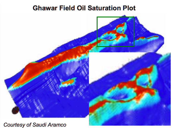
Here the question is: is this an accurate picture of the state of recent depletion of Ghawar? (Ghawar is the world's largest oil field, and source of over half of the oil produced by Saudi Arabia). And if so, then the second question arises: does that depletion have anything to do with this picture?
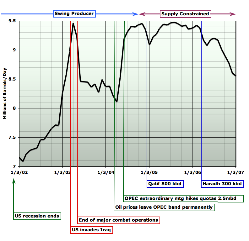
In particular, Saudi oil production has been falling with increasing speeed since summer 2005, and overall, since mid 2004, about 2 million barrels of oil per day in production has gone missing (about 1mbpd in reduction in total production, and about another 1mbpd in that two major new projects, Qatif and Haradh III, failed to increase overall production). That's 2.5% of world production and, if that production hadn't gone missing, gasoline in the US likely would still be somewhere in the vicinity of $2/gallon instead of well over $3. I will analyze six or seven separate lines of technical evidence, and argue they all point to a consistent picture, which says that the answer to both questions is "Yes". Yes, the northern half of Ghawar is quite depleted. And yes, this probably explains at least part of recent production declines. Furthermore, it is likely that more declines in Saudi production are on the way. The evidence in question comes from quantitative forensic correlation of hundreds of disparate pieces of data from dozens of technical papers about different aspects of Ghawar. Thus this analysis is very long and detailed - my apologies to the reader. It summarizes 300+ hours of work on my part, and probably similar amounts of work by several other members of the loose Oil Drum coalition investigating Ghawar and (most particularly Euan Mearns, who has posted his own thoughts and Fractional_Flow). It's just a lot of material to document. And in attempting to address both the detail needed by technical readers and the explanations needed by less-technical readers, the length has grown further. Given the importance of the subject, in a choice between being thorough and being brief, it seemed better to be thorough. I will at least do my best to be clear in my exposition.
The Linux Supercluster PictureLet's first go over a little background to make sure we understand what we are looking at. We'll start with this schematic of part of Ghawar (courtesy of Euan Mearns):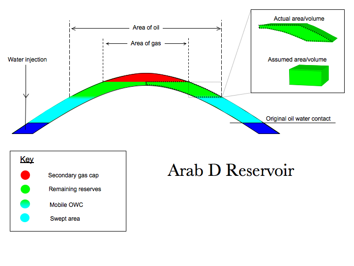
An oilfield consists of some layers of rock, the reservoir, which contain pores, spaces between the rock grains, which contain some combination of oil, water, and natural gas. Above the reservoir is a cap of some kind which will not allow the passage of fluid and which is shaped to trap the oil and gas from migrating upwards. This they otherwise would do because they are lighter and more buoyant than the water that tends to fill rock pores underground. Roughly speaking, the green volume in the picture above is the oil, and the dark blue volume is the water that was originally below it. This is not quite true, as the oil region invariably has some droplets of water still trapped in the rock pores as well: this is the initial water which cannot move. There may or may not be a cap of natural gas above the oil, depending on which part of the field we are in. Oil in Ghawar is being produced by peripheral water injection. In this case, in addition to the natural water below the oil, water is being pumped down special injector wells at the edge of, and thus below, the oil area. The pressure of that water is slowly forcing the oil up the structure to wells at the top, from where it flows to treatment plants. The pale blue area in Euan's picture above is the swept area that used to be oil, but now is mostly water. Unfortunately, it's not all water. Just as there was some water in the oil before we started, there will be some oil in the water when we are done. This residual oil, which will not come out from any amount more flooding by water, consists of little droplets of oil beaded up and stuck in small pore channels in the rock. So with that understanding, let's look at the Linux supercluster picture again. By default (or if you click the "Region Labels On" button), we are looking at labels of the division of the field into major operating areas. For readers new to the subject, it will be particularly useful to take a minute to become familiar with these.
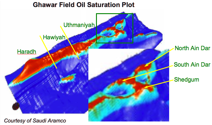 "Linux Supercluster" visualization of oil saturation in Ghawar, with focus region on 'Ain Dar and Shedgum regions at northern end. Use buttons to cycle labels. Source: Figure 3 of Linux Clusters Driving Step Changes in Interpretation Simulation. (pdf).
If you now click the "OWC Labels On" button, you will see labels that show, for the northern operating regions, where the contact between oil and water was before production started - the original oil water contact (OOWC). I've also shown as "OWC2004?" the approximate level of the oil water contact (OWC) at the time the picture denotes (perhaps 2004), and, in yellow, the crest of each structure, which is where the water will reach to when all production by waterflood is over. At that point, this picture would show those "hills" as all pale blue (at least if all oil could successfully be produced). As you can see, the picture shows quite a lot of the "hills" already being free of oil. Although it's hard to estimate precisely, I don't think you could say that the average height of the top of the pale blue swept area has reached less than 55% of the height of the structure. Similarly, I think it's definitely less than 75% of the way up - overall it looks about 2/3 of the way up. I encourage you to stare at the picture and make your own subjective estimate to see if you think my range is reasonable - I will be comparing this to other estimates later. However, something that's important to understand about this picture is that the vertical scale is very exaggerated to make the shape clearer. Ghawar is really enormous and almost flat. It's about 175 miles from tip to toe (ie 2 1/2 hours driving at freeway speeds). And the structure slopes up to the center at only a few degrees. The effect of that is to make it so that 2/3 of the way up the structure is a lot more than 2/3 of the oil gone. This next picture shows a model estimate that I generated (explained later) of the effect of being two thirds of the way up in the 'Ain Dar and Shedgum regions. On the left is how much oil was there to begin with (darker red is more oil) and on the right is how much would be left (roughly) if the OWC were 2/3 of the way up the structure like that.
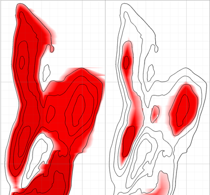
The model doesn't quite distribute the oil the same as the Linux supercluster picture, but it's in the ballpark, and because it allows you to effectively look straight down, you can see how much oil has gone. We will discuss exactly what this model is doing later. For now I just want to illustrate that 2/3 of the way up the structure is a lot of oil gone. However, after all this discussion of the Linux supercluster picture, you might be wondering whether there's any reason to think it has any fidelity to the true state of affairs in Ghawar. The paper from which the picture comes is a general survey for an industry magazine of the use of Linux superclusters for large scale computation tasks in the oil industry. The authors discuss as one of their examples Saudi Aramco's use of these types of massively parallel computing clusters to simulate oil and water flow in their reservoirs:
One approach is to not make the assumptions. Instead, brute force can be used to run very large simulations where the best geological understanding is rendered in detail. Already, models run at higher resolution than in the past. In the case of managing the world's largest asset, the Ghawar Oil Field, Saudi Aramco runs its POWERS simulator on a massively parallel HPC. As of 2004, this 128-node Pentium IV�-based machine had run full field simulations with between 10 million and 100 million cells and more than 4,000 wells, with larger runs pending. These simulations are run with multicomponent hydrocarbon models, waterflooding with varying brine chemistries, and dual-perm response to match fracture-flow history. Some runs include CO2 floods.And that's all the text covering Figure 3. So, clearly the picture is not intended as a report on the status of Saudi fields. Instead, it's intended as an illustration of how cool their simulators are. The question is, did Saudi Aramco a) accidentally publish to the entire world, in an obscure publication, a state of the art simulation generated picture that revealed very clearly the status of their biggest oil field as of 2004 (the year that the text references simulations as being done)? Or b) give away a simulation of some other year, maybe far in the future, or some hypothetical scenario that bears no relationship to current reality? Clearly, the question cannot be answered beyond reasonable doubt from the text above. So now we will turn to other evidence. First, however, we will have to gain a better understanding of the nature of the reservoir, so that we can better understand that evidence. Before moving on, I want to briefly draw attention to the mention that some simulation runs "include CO2 floods". This suggests planning for tertiary recovery approaches (low production rate, expensive, final resort ways to get the last oil out of a field).
Geology and Reservoir PropertiesThe structure of Ghawar is a large anticline - the compressive forces of plate tectonics have caused the almost level strata of sediments to buckle up very slightly. The reservoir rock, which is known as the Arab D layer, was laid down in a large shallow sea off the Arabian coast during Jurassic times. It is essentially limestone formed of the remains of countless marine organisms that lived in that sea, died, and fell to the bottom. In places where the sea was shallow, storms and currents stirred up the sediments and ensured that only larger grains could stay in place - these ultimately formed highly porous rock which could hold a lot of fluid (high porosity), and in many cases allow that fluid to flow freely amongst the pores (high permeability - related to porosity, but not the same thing as sometimes ample pores can be poorly connected to one another). In other places, deeper waters allowed the deposition of very fine particles which formed lime mudstones with limited pore space and even poorer flow properties.Overall, the sea rose at the beginning of the deposition of the Arab D reservoir, and so the rocks at the bottom are poorer in reservoir qualities throughout the field. As the sea gradually filled up with sediments over the course of 2-3 million years, it got shallower and the rock formed grew more porous. Thus the rocks at the top of the reservoir are generally better. However, the southern end of the reservoir was generally deeper water than the northern end, and the rocks there were substantially poorer even in these later stages. However, considerable briefer variations happened at one time and another and there is significant vertical and lateral heterogeneity in the rock. We can summarize the situation though by saying that there is about 250'-330' of total Arab D rock, with more at the northern end. Of this, 140'-200' were traditionally considered sufficiently permeable to allow oil production, and constituted the "net pay". The bulk of the net pay occurs in the upper half of the strata - generally known as Zone 2 - but the balance occurs in a number of thinner layers scattered through the lower zone 3, and even into the rarely discussed zone 4 at the bottom. Eventually, the deposits climbed high enough and the sea retreated enough that the top of Ghawar became a large salt flat, which eventually formed into a thick impermeable layer of anhydrite. Thus later, when oil from slightly older deposits began to rise up through fractures in the rocks below the Arab D reservoir to replace some of the water there, it encountered the anhydrite layer and could go no further. Zone 1 is a transitional zone between the high quality zone 2 layers of reservoir and the overlying cap which will not support fluid flow at all. To get a clearer sense of the zones have a look at this next picture (you might want to click on it to get a larger version in its own window). This shows the porosity, permeability, and rock type as a function of depth in one well somewhere in the Uthmaniyah region of Ghawar (the paper from which it comes does not give a more precise location).
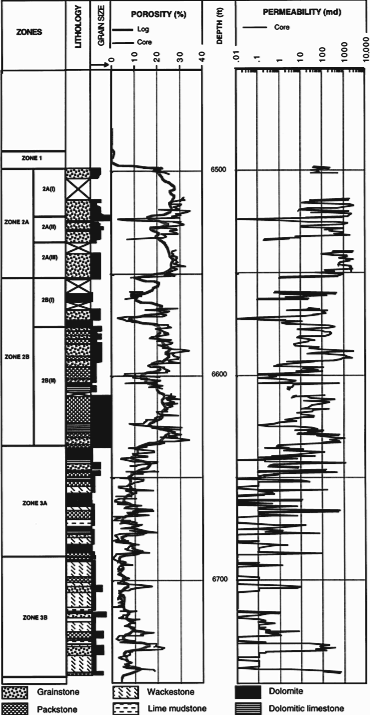
As you can see, there is about 250' of total (ie gross) reservoir in this well, and you should be able to see the clearly higher porosity and permeability in zone 2 versus zone 3, especially the upper part of zone 2 (we will discuss porosity and permeability more quantitatively later, but it might be worth noticing now that the permeability is on a log scale). For another perspective on the situation, take a look at this next figure which comes from a 1962 analysis by RW Powers of Ghawar rock (with some reconstruction by me). This is how the figures were originally created from samples taken every six inches from an oil well, and then mounted on 1200 microscope slides:
A standard Leitz mechanical stage was converted to a point-stage by addition of a spring clip to engage notches filed in one of the traversing wheels. These notches were spaced to allow a linear slide motion of 0.8 mm between stops. Distance between point count lines was controlled by the second traversing wheel. Numerous experiments were tried to determine an ideal spacing between lines of points for obtaining acceptable results in a minimum of time. Initially a pattern with points 0.8 mm and lines of points 1.0 mm apart was used (about 600 points per slide). Compared with line integration results from the same slides, this point density gave no difference for any one constituent greater than 2 per cent. Using a 0.8 by 2.0 mm grid on slides with irregular particle shape and poor sorting, the maximum difference was 4 per cent. The difference increased progressively as distance between traverses increased. Most slides were finally counted on a pattern of 0.8 by 2.0 mm (about 300 points)...1200 slides, 300 points each, bent over the microscope, click, measure, click, measure, click, measure, day after day, week after week, month after month. Heroic science. All I did was cut and paste his figures together and then measure various things in them. This is a log from a well in Haradh (the southernmost, poorest part of the field):
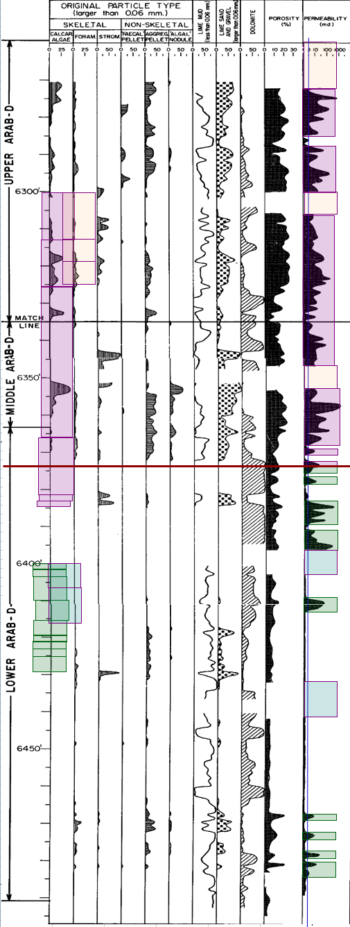
Here we have only about 205' of gross reservoir - significantly less than in Uthmaniyah. The colored boxes represent an analysis to determine the amount of net pay (defined here as rock of permeability 3 milliDarcies or better (anonymous industry experts assessed the boundary between "net" and "non-net" as anywhere from 10mD to 0.3mD, and report that over time the trend has been to count worse rock as included in the reservoir, a point we will return to). You can see that zone 2 has a lot more net pay (the pink boxes) than zone 3 (the green boxes). This well has an estimated 136 feet of net pay. (The "estimation" comes into it because we have to correct for missing data). Hopefully, the gradient from Uthmaniyah down to Haradh is clear. Everything is somewhat worse - there is less zone 2 in total, less of both zone 2 and 3 are "net", the net there has worse porosity and permeability. Wells further north than Uthmaniyah are roughly of similar nature, but a bit better: they have more zone 2, more net pay in both zones 2 and 3, and the net pay is better (more porous and more permeable). It's also worth noting the enormous variations in the permeability, which is shown on a log scale. Rock of permeability 1000mD will, at the same pressure difference, carry 1000 times more fluid flow than rock of permeability 1mD, and both extremes are common in the Ghawar reservoir rocks - the reservoir is not homogeneous at all, even in a single well. Porosity varies in the range 5% to 30%, though the upper end of that range is not attained in this Haradh well. If you study this next picture, it shows a series of well summary pictures from Powers 1962 paper, with the Zone 2 and 3 net shown in overlaid colors (I determined the correspondence between the modern zone 1-4 scheme and Powers upper/middle/lower scheme by detailed correlation of wells in Uthmaniyah - the bottom of his "Middle" cuts off about 10' above the bottom of zone 2 in Uthmaniyah). I cut and pasted Powers pictures together into a north-south spectrum of just the wells he analyzes in Ghawar. Click on the picture to get a bigger version in its own window:

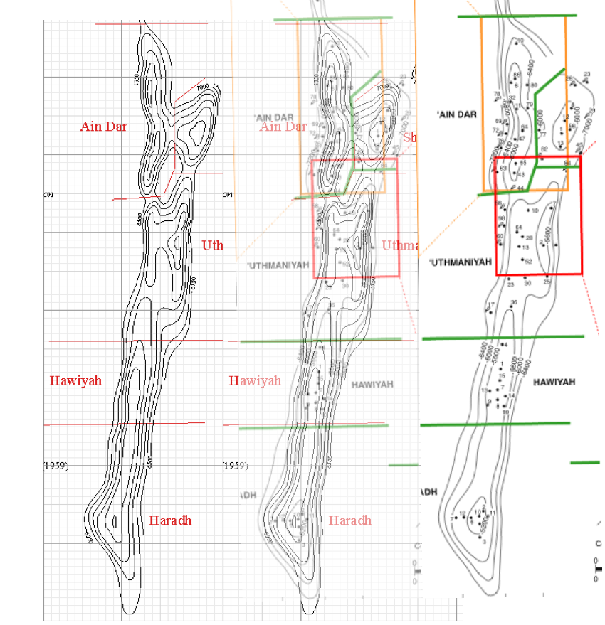
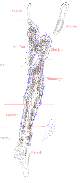
In addition to the trend in the amount of zone 2 to zone 3, you should also look at the "Calcarenitic and coarse carbonate clastic" component. That's the good stuff: big open grain structure that will let lots of fluid flow. You will see that there is far more of this open grained rock in the north than the south. There is also more in the upper part of the wells than in the lower. Thus it is that the rock in the south is significantly poorer than the rock in the north, though this is a continuum, rather than a fundamentally different kind of rock. The largest depth of gross reservoir in any of these wells is about 270-280'. However, in the literature there is discussion of as much as 300'-330' of reservoir when the very poor quality Zone 4 is included (zone 4 is frequently not mentioned or studied, presumably because it makes a very limited contribution to production in most locations in Ghawar). The approximate location of the wells in that last picture is as follows:
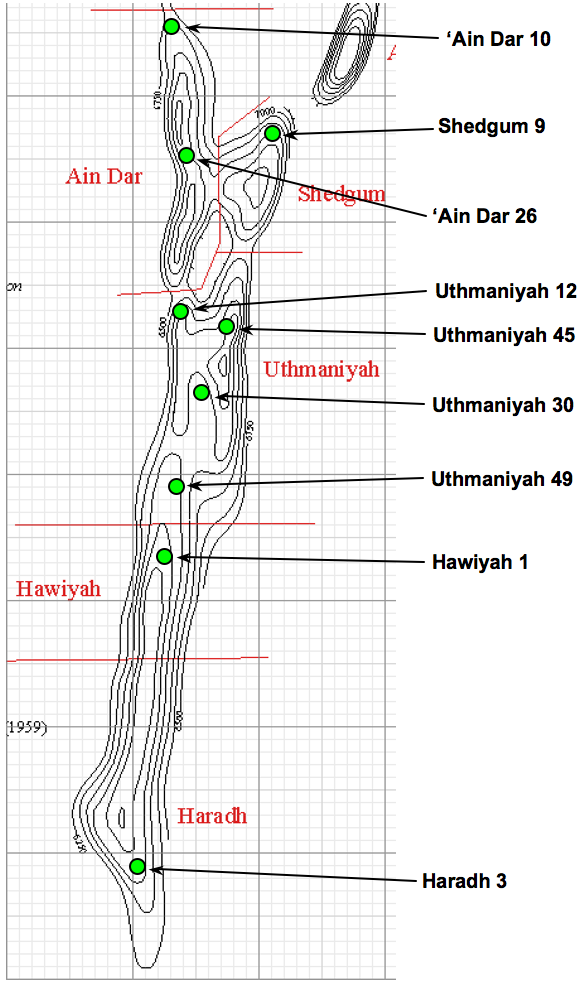
As you can see, they form a reasonable sampling of the field, though not as good in the south as the north.
Development History of the FieldLogically enough, the development of the field began with the good parts in the north and has gradually proceeded south. Ain Dar, Shedgum, and Uthmaniyah all began production in the 1950s, Hawiyah not until the 1970s, and although there was some limited development earlier, full injection supported production in Haradh has been bought on in three phases - Haradh I in 1996, Haradh II in 2003, and Haradh III (the "toe" of the "boot") only in 2006.An anonymous correspondent recently gave me a hard copy of the 1979 staff report to the US Senate Subcommittee on International Economic Policy on "The Future of Saudi Arabian Oil Production" (the report mentioned in Appendix C of Matt Simmons' book "Twilight in the Desert"). It has the first reliable figures for plateau production in all the operating areas that I have seen. At that time, production was as follows (either actual or planned):
The figures for Hawiyah/Haradh were planning assumptions, not based on actual production. We know from a recent paper that Haradh produces 300kb/d from each of three operating areas, for a total of 0.9mb/d. Production of 0.4mb/d in Hawiyah would look about right as it has similar area to South Uthmaniyah, about half the area of Haradh, and quality intermediate between those two. We will discuss more recent production history in a little while, but this gives a sense of the relative importance of different areas. The important point is that the northern end of the field, from North Uthmaniyah up, has historically been far more productive, with over 2/3 of the productive capacity on these figures. The combination of more rapid production and a much earlier start to production would certainly make it plausible that these areas of the field would become depleted first.
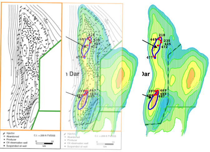
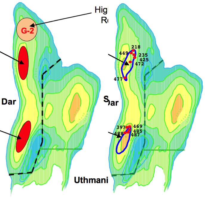
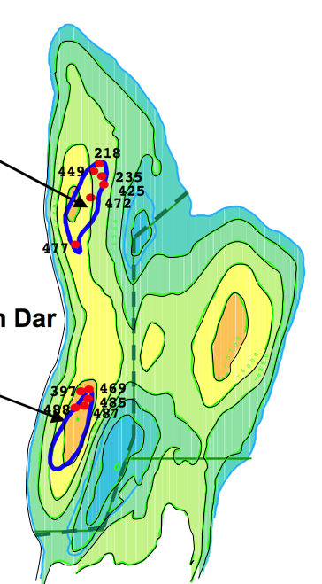
Evidence of Recent Flood Front Location in South 'Ain DarNow that we have a feel for what the reservoir rock layers are like, and the different operating areas of the field, we are in a better position to assess various other pieces of evidence for the position of the flood front in recent years.The first piece of evidence comes from a paper by Hussain et al Optimizing Maximum-Reservoir-Contact wells: Application to Saudi Arabian Reservoirs presented to the 2005 International Petroleum Technology Conference (IPTC 10395). The paper is a discussion of several well planning exercises in Ain Dar and Shedgum. Individual simulations were performed to assess the likely lifetime performance of the wells. However, our immediate interest is in a picture which shows the location of one of the planned wells:
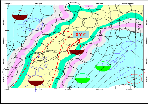
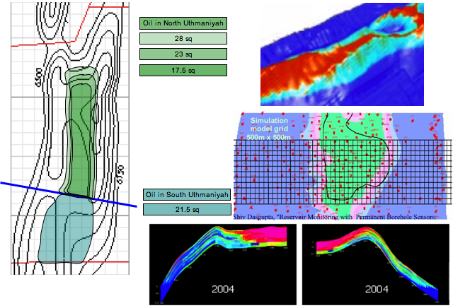
There is no key for this figure in the paper, and nor is the location shown in terms of the rest of the field. Thus, the first time I looked at this it seemed completely mysterious. However, after staring at it long enough, it turns out it can be decoded to determine quite precisely the state of the field in South 'Ain Dar and the saddle between South Ain Dar and Shedgum. The key thing is to look at the contours. I have labelled them more clearly, and shown the relationship to an overall map of 'Ain Dar/Shedgum, a key to the oil layer from Figure 8 of the same paper, and the relationship to the Linux Supercluster picture.

Let me try to explain what you are looking at here. Firstly, it's critical to understand what the contours mean. These are depths below sea level in both Figure 11 and the fragment of the map from Greg Croft's page (on which much more later). The contour heights refer to the top of the Arab-D reservoir. So when looking at a point on the 5800 contour, say, we are looking down on the top of a column of something like 275' (give or take) of reservoir rock. Since the top of the reservoir at that point is at 5800' below sea level, the bottom of it would be at 6075' (in round numbers). Of that 275' of reservoir or so, about 200' or is actually good productive rock, while the rest is marginal enough that, at least in the past, it would not have been considered, but the 200' of good rock is scattered in layers amongst the total 275' of rock column. Within the context of a small area like Figure 11, the thickness of the reservoir probably doesn't vary much. In particular, any variations in structure thickness probably don't have much to do with the variations in structure height, since the thickness is controlled by events when the rock was being laid down in the late Jurassic, while the height is controlled by tectonic distortion of the structure during the Cretaceous, 80 million years later. Now, if you look at the location for Fig 11 (100' contour interval) I have proposed in the overall 'Ain Dar/Shedgum picture (250' interval), hopefully it is clear that there is really no other candidate location that could work at all. To get those contours to match, you have to be high up on the south side of a east-west saddle that tops out at a little below 6000'. There's only one place like that. Once you've got your mind around the contours, the next thing to look at is the colored regions, which almost certainly represent the thickness of the oil layer, with yellow representing something close to the original thickness of the layer, and the other colors representing less and less thickness of oil (because water is intruding into that part of the oil layer as the water advances and the oil retreats up the structure to be produced out of wells up there). A key from Figure 8 of the same paper, which shows a well location in Shedgum is included above, and this figure likely has a similar color scheme. So, given that, it should be clear that the picture above is similar to the Linux Supercluster picture. A relatively narrow ribbon of oil lies along the top of the south 'Ain Dar cap and goes across the saddle to Shedgum, while a much narrower ribbon goes up towards the North 'Ain Dar crest. On the crest, there is no oil column below the 5900' contour, and we don't have a full column below 5800'. However, the oil across the saddle dips down, and we have a full column crossing the saddle down at some level between 6000' and 6100' below sea level. Back before oil production began, oil in this area went down a little below 6500', while the top of the South 'Ain Dar crest is a little shallower than 5600 feet. So overall, we are about 2/3 of the way up the structure on the crest here, but have some extra oil in the saddle. So this is very much consistent with the Linux Supercluster image being a 2004 image (given this Figure 11 is from a 2005 paper).
A Word on UncertaintiesBefore we go much further, I want to say a few words about errors and uncertainties. One of the things I have attempted to do in this analysis is to make quantitative estimates of the uncertainty in all the important things I am analyzing, and you will be seeing more and more of this from here on out. Some folks who saw early drafts of parts of this analysis experienced some confusion if they don't think this way all the time, so let me stop here for a micro-lecture on that subject.When I say, as I will shortly, that I believe the ultimate recovered reserves (URR) of oil from Ghawar via waterflood (that is excluding tertiary recovery techniques) will be 96 ± 8 billion barrels (gb) of oil, that could be translated informally as follows:
More formally, in a wide variety of practical situations, the results of a complex calculation that brings together many different unrelated uncertainties will be approximately "normally distributed" - having a special mathematical form originally due to the German mathematician Gauss. If so, then we can say that the odds of the end result being no more than "one sigma away" from the estimate is 68%. The probability of being no more than two sigmas away is 95%, and the probability of being no more than three sigmas away is 99.7% - that is there is only 3 chances in a 1000 of being more than three sigmas from the estimate if that estimate and uncertainty were correct. If the assumption of a normal distribution is in serious doubt (which I don't believe it is here), then a pretty much universally applicable theorem called Chebyshev's inequality guarantees us that the worst case is that the two sigma range is at least 3/4 probable, and the three sigma range is at least 8/9 probable. Where possible, I have estimated uncertainties in various quantities by using some type of sampling or statistical procedure. In some cases, that is infeasible. For example, we presently estimate the amount to oil in Uthmaniyah by combining three pictures visually. This is necessarily a somewhat subjective procedure. In those cases, I make three estimates: the value that seems to me most likely, the value that seems the least that could possibly be the case, and the value that seems the most that could possibly be the case. I then take the average of those values as my estimate, treating the range from the smallest estimate to the largest estimate as the two sigma uncertainty range. In practice, such estimates work well when combined with a number of other independent uncertainties. There are well established mathematical rules for combining uncertainties, which I have employed. For example, let's look again at the picture above of South 'Ain Dar, and try to use the less formal procedure to estimate the average height of the oil water contact, and an uncertainty in the average.

My read on the picture is lowest conceivable: 6100', highest conceivable: 5900', likeliest, 6000', so I would quote 6000 ± 50'. Note the latter is intended as the one-sigma uncertainty in the average, not the range of variation which would clearly be greater. To compare, I then took the first 20 in a list of randomly sampled locations in the picture, and, on the assumption that the color scale runs from zero to 275' ± 25' of gross oil layer above the water, I obtained an average and standard error of 6032' ± 38'. So the two estimates agree within error bars, though the latter is likely a little better estimate.
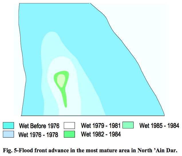
Flood Height in North 'Ain DarNext, we turn to a more complex line of evidence that comes from the 2005 paper on water management in North Ain Dar (SPE 93439). A number of figures in that paper provide data that we can interpret to constrain the position of the OWC in 2004 for comparison with what we have inferred so far.The first is this picture:
They don't spell out for us where this picture is, but the outline can be fitted nicely into better maps that have contours:
From this, I estimate the following heights for the OWC at different times:
Next, there are several sources that, taken together, allow us to establish the rate that the OWC (oil-water contact remember) has climbed since. For example, there are flowmeter profiles for three different wells in Figure 8. Each of these shows the cumulative percentage of fluid as a function of depth in the well, with green being oil, and blue being water. As you can see, typically the water's contribution is in the bottom of the well, and the oil in the top. The dividing line is the oil water contact in that well, and it rises over time.
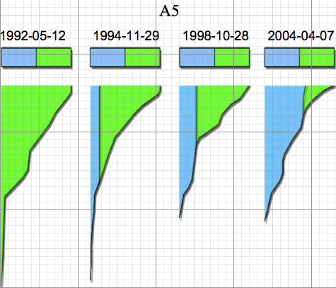 Flowmeter records for three wells in North 'Ain Dar (click buttons to switch wells). Position of flood front was estimated using grid and highest location in which water is emerging from well (as indicated by a right edge to the blue region that was not vertical). Source Figure 8 of SPE 93439
Now, we don't know the exact depth of these wells (no depth scale is provided), and we don't have an a-priori reasons to suppose they are all the same depth, but the form of the profiles, with copious production from the upper half to two thirds and much smaller production in the lower one third to one half suggests that we have all of zone 2 and most or all of zone 3. It doesn't appear we have zone 4 or the copious zone 2 production would make up less than half of the profile. If we thus assume we have 250' of depth in all cases, and then plot the resulting depths versus time on a common graph, the overall agreement is quite striking: 
In addition to the three well curves (with linear fits), I have added a blue line, which is in an arbitrary vertical position on the graph, but the slope of which is determined by translating the average 5.096 feet/day horizontal flood front velocity from this next graph in the same paper to a 0.0505 feet/day vertical velocity by assuming the original velocity was a southward velocity up the North 'Ain Dar ridge. The agreement with the velocities determined from the well flowmeter profiles is excellent. This is a striking illustration of the power of correlation to extract useful information from noisy uncertain data.
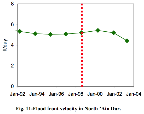
The combination of all this evidence gives an average vertical velocity of the flood front of 18.4 ± 0.7 feet/year over the period during which it was linear. So we can start at the locations back in the late 70s from figure 5, and extrapolate forward at this rate. This next picture summarizes everything we know so far about the level of the oil water contact over time in North 'Ain Dar. 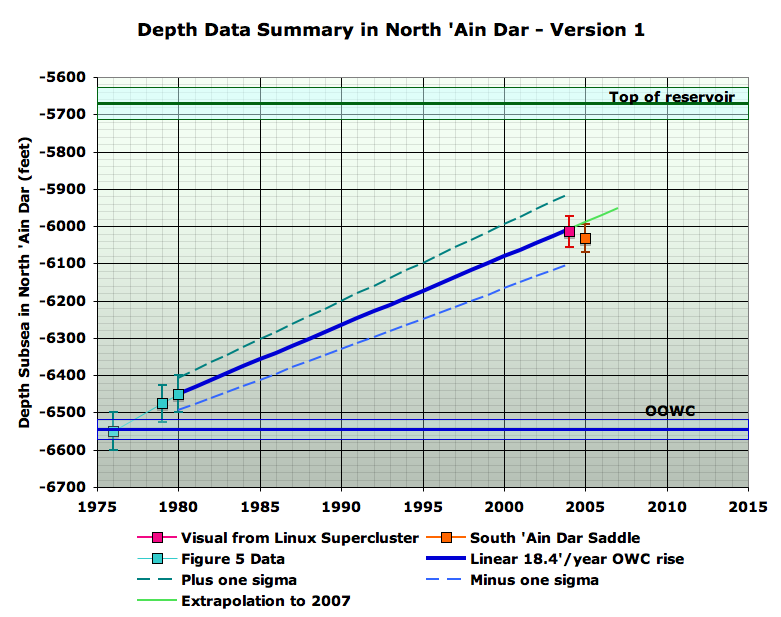
Starting at the left, we have, in turquoise, the SPE 93439 Fig 5 data for the far northern end of the northern 'Ain Dar ridge in the 1970s era. Then we have the fairly constant 18.4' vertical feet/year march up the ridge from the Fig 11 flood front graph and the Fig 8 flowmeter profiles in the same paper. Then, the pink point comes from translating the subjective visual estimates from the Linux Supercluster picture that I gave earlier. Finally, we have the orange point being the South 'Ain Dar saddle estimate from sampling the IPTC 10395 Fig 11. Hopefully, you will agree that a pretty consistent picture is starting to emerge from this various evidence. I haven't told you yet why I think the OOWC (original oil water contact) is where I show it, and you might also wonder why the OWC was still at the OOWC in 1976, when production in this operating area began in 1951. Hold those questions for a couple of sections. It's time we started to talk about how to estimate how much oil is in these fields, and that will eventually clarify these points.
Framework for Understanding VolumetricsSo the procedure for estimating how much oil a given field might produce, or how much might be left at some point, is conceptually simple. We need to know the volume of rock in the reservoir, what percentage of that rock is pore space (the porosity), and what percentage of that pore space is occupied by oil, versus other fluids (the oil saturation). Porosities of the Arab-D reservoir rock in Ghawar can range from a few percent up to as much as 30% or so. One other wrinkle is that the oil will shrink as it comes out of the ground (due to natural gas coming out of solution in it), and we care about how much oil there is after it has done this. This shrinkage factor is known as the formation volume factor. So if we multiply these four numbers together: rock volume, porosity, oil saturation, and the inverse of the formation volume factor, then we will know how much oil is in the ground at some given time, if it were brought to surface conditions.Some more complications arise. The simplest way to assess the volume of rock would be to measure the area on a map of the reservoir, and then multiply that area by the average thickness of the reservoir rock. But to be more accurate, we will need to understand the shape of the reservoir in three dimensions. Borrowing Euan's nice picture again, we can illustrate the general idea in cross section:

In the case of Ghawar, the main complication arises from the triangular wedges where the oil runs into the water (ie the oil water contact), which can be several miles wide. When I said "roughly speaking", one of the issues of interest is that not all the porosity in the green zone is full of oil that can come out. Firstly, it is never the case that pores are 100% filled with oil even in the reservoir at the outset. There is invariably at least a little bit of water in there too, clinging as tiny droplets stuck inside little pore channels somewhere deep in the rock. The fraction of such water is known as the initial water saturation. Better, more open rock, will have lower initial water saturation, particularly if it is a long way above the oil water contact. In that circumstance, the water saturation might start out as low as a few percent. However, in very poor quality rock in the transition zone near the water, water saturation can start out as high as fifty percent even in an area that is nominally oil. All cases in between occur. Furthermore, after the flood front has passed by a given piece of rock, and water has been washing through it for a couple of decades, there will still be oil left in that piece of rock, again in the form of droplets trapped inside pores that cannot move. This oil cannot be produced by waterflood alone - if it ever comes out it will be because of additional (ie tertiary) recovery techniques, should such prove economic. The fraction of rock so occupied by oil at the end is known as the final oil saturation (and the fraction occupied by water is the final water saturation). Thus, in a given barrel of reservoir rock, the fraction of the barrel that will end up as oil on the surface is given by the porosity percentage (how much pore space there is to hold fluid of any kind), multiplied by the difference between the initial and final oil saturations, divided by the formation volume factor that controls how much the oil will shrink by the time it gets to the tanker. The remaining wrinkle is the net/gross distinction we briefly discussed earlier. Fluid in the reservoir during production moves because of pressure gradients. The injectors are increasing the pressure below the oil, and this is exerting force on the oil to move upwards and towards the producing wells. However, the amount of movement that the oil makes in response to a given pressure difference depends on the permeability of the rock. As we discussed earlier, this is related to the porosity, but not perfectly so. In some rocks, the pores are poorly connected with one another, and it is hard to force fluid through them. In others, the pores are well connected and fluid flows more freely. Now, some rock has such poor permeability that, even though it contains some oil, that oil will not come out of it in any reasonable period of time. Flow time is measured in centuries rather than the years-decades required to meaningfully contribute to the oil production. Oil geologists and petroleum engineers distinguish net pay from gross reservoir. The former excludes the not-sufficiently permeable rock, whereas the latter is everything. Typically, there are layers of pay interspersed with non-pay, and this is very much the case in Ghawar, as we saw in the well logs earlier. However, the distinction between pay and non-pay has been shifting over time. The only data on this comes from Euan and I asking our networks of anonymous industry advisors. We got answers ranging from 1mD to 10mD for the 1980 timeframe, but also a statement that at least one company (that you've heard of) will sometimes now consider rock down to 0.3mD as pay, given better technology to access such poor rock (and, perhaps, lack of enough better reservoirs to drill into, meaning companies can't afford to be too picky). The main technology enabler has been precise geo-steered horizontal wells, allowing wells to be drilled horizontally along the low-permeability layers, from whence the oil will slowly drip. These variables tend to be loosely correlated. Rock of higher porosity is more likely to be permeable, and more likely to have a low initial water saturation. In short, it is "good" rock. "Bad" rock has less pore space, poor flow properties even in the limited space there is, and high water content at the outset.
With that background, let's now turn to the available map data, which is one critical component of the volumetric oil estimation we will do.
Euan reported the large industry report map to have a considerably longer Ghawar than the Croft map. Careful measurements based on same contour analysis do not support this. I find the distance from the bottom of the 6000' contour in Haradh to the 6400' line in North Ain Dar to be 143.7 miles in the Croft map, and 140.7 miles in the industry map, a variation of only 2%. My best reconciliation of the two maps, on identical scales, looks as follows:
This does not show an overall systematic scaling error between the two maps in my judgement, but many local variations in the exact structure (note to others trying to work on this problem: it's very important to compare contour-to-contour, not just look at the overall outline, since one map has contours going deeper than the other). Clearly, at least one of these maps is somewhat imperfect. An analysis of the more detailed map of 'Ain Dar turns up more serious problems however:
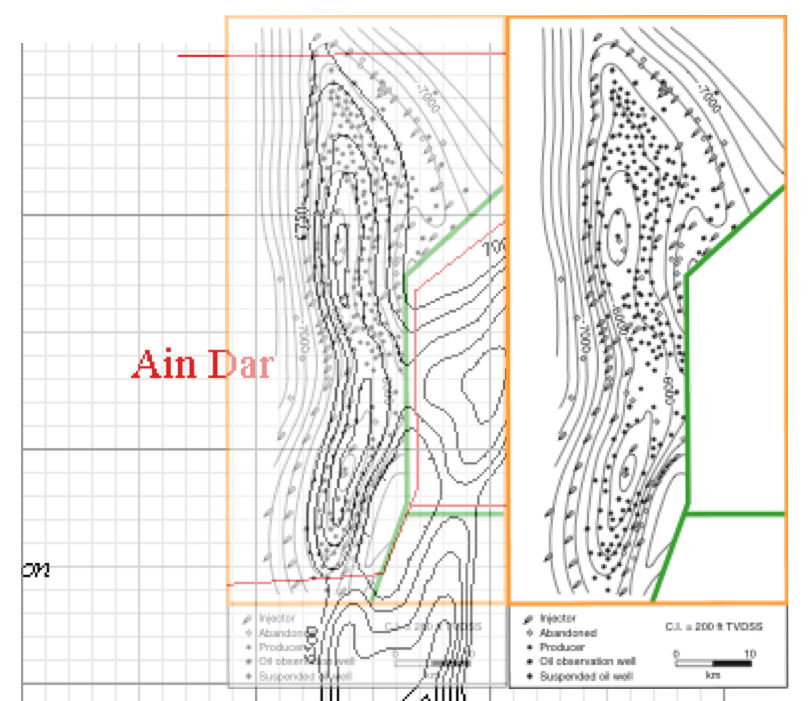
Even on a equal-contour basis, the industry report map has significant areas above the oil water contact line that are not in the Croft map. This is especially problematic in North 'Ain Dar, where I estimate the area difference to be about 50% (Euan suggested 25%). Euan's reconciliation of the well location map with the Croft map suggests the same issues apply to Shedgum. For this reason, I decided to use the asphaltene map for estimates in 'Ain Dar and Shedgum. This map reconciles quite well with the industry report map:
Both appear to be more modern accurate maps. The industry report map has a scale, and this was used to establish the scale for the asphaltene map, which is not provided with a scale in Saudi Aramco papers I have seen. I did the reconciliation twice on different days and only came out 1% different in the resulting scale, an error which is negligible compared to other uncertainties in the problem. In the rest of the field, I used the Greg Croft map. However, reconciliation of the Croft map with the asphaltene map suggests Croft is about 20% too narrow in Uthmaniyah. The approach I have taken to this overall problem is to correct reserve estimates for Uthmaniyah upwards by 20% and to view all regions estimated with the Croft map as having a 20% map uncertainty in their reserves. No corrections were applied to Hawiyah which seems to be about the right size. The special problems in Haradh are discussed later.
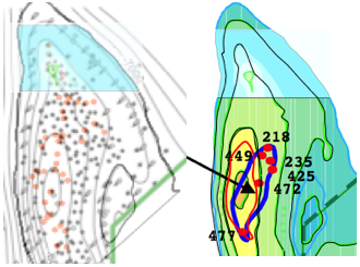
Modeling the StructureAs part of this analysis, I wrote a C program to parse an image of the map contours, and for each of the Croft map and the asphaltene map, used it to build a three dimensional model of the reservoir based on the map. This formed the foundation of my estimates of oil reserves and depletion. I linearly interpolated between contour lines, and where I had indications that the oil extended outside the structure in the map contours, I extrapolated from the last two contour lines on that edge of the structure. I placed the top of each crest midway between the lowest contour that no map showed for that crest, and the highest contour that any map showed for it, and linearly interpolated up to that point (ie my crests are conical in the last 75-125').While we will cover more aspects of this modeling as we go forward, this montage should give you some feeling for the kinds of things the code has to do, and hopefully provide visual evidence that it works correctly:

Since my code parses these maps and counts each pixel to estimate area, and since each pixel represents a small fraction of a mile, errors due to digitization of the map are negligible. The way I do linear interpolation introduces a small amount of noise between contours that is different than the noise the real structure would have. This is expected to be small compared to other errors (it's more a visual issue than anything).
Original Oil Water ContactIn order to estimate the volume of oil-bearing rock reliably, we don't just need the map, we also need to know where the oil is, and where the water is. That is, we need to estimate the position of the oil water contact, which forms a surface that intersects the base of the reservoir. You might imagine that the oil water contact would form a level plane, but in fact it is tilted and somewhat uneven. The main reason for this is that the water under the oil varies in its density because of large changes in salt content in different parts of the reservoir. The approach I took to this issue was to fit a tilted plane to available data on the position of the oil water contact. The regression (model fit) provided estimates of the uncertainty in original oil water contact (OOWC) position.Let's first take the case of the Croft map, which was used for estimates of original reserves in the south of the field. Estimation of the position of the OOWC (original oil water contact) was carried out as follows for areas other than Haradh. The map showing OOWC estimates in the 1959 Aramco AAPG paper was reconciled with the Croft map as follows: 
The regression resulted in a plane that has the following characteristics:
Haradh is known to have its own local OOWC tilt dynamics that are more pronounced than the rest of the field, and furthermore, the 1959 OOWC measurements constrain the Haradh OOWC only very weakly. The best available data come from SPE 71339 by Stenger et al and titled Assessing the Oil Water Contact in Haradh Arab D. The following is a reworking of their Figure 10, with a reconcilliation of the Croft map, and annotations in blue of the absolute depths based on the text of SPE 71339. Estimation of the position of the OOWC (original oil water contact) was carried out as follows for areas other than Haradh. The map showing OOWC estimates in the 1959 Aramco AAPG paper was reconciled with the Croft map as follows: 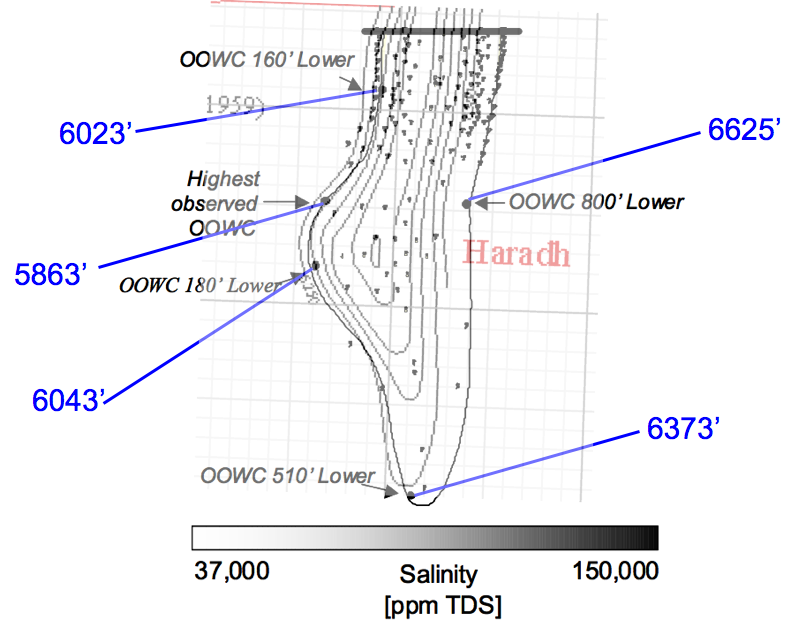
Stenger proposes that the main explanation for the uneven oil column is the presence of very saline water under the oil in the east, and a localized source of much fresher water in the west, close to the point of highest oil contact.
It did not seem practical to base an interpolation model for the depth on these data - clearly any linear model will fail badly, but the data are inadequate to suggest what kind of non-linear model would be suited. It appears that the main effect of the OOWC is to add to the oil filled area to the east of the Croft map. Accordingly, we treated this issue by adding a 20% upwards correction to the Haradh original reserve estimates, with ten percentage points of uncertainty. Turning now to the northern areas of the field, we use the ashphaltene map shown to the right. Splines were fitted to the contours, and these splines were parsed to generate a three dimensional model. The map shows the oil water contact as the blue line around the edge of the map, or in places, in the interior of the structure. The regression fitted to depths inferred from this blue line, has the slope of 2.5 feet downward for every mile to the north and 6.6 feet downward for every mile to the East. The r2 of the model was 48%, and the uncertainty in the vertical height was 23 feet (in other words, compared to the whole field, the regression in just the northern fields finds less systematic height variation, less uncertainty in the height of the contact, and so a larger fraction of the variation is noise, rather than systematic trend. This map is believed to be quite accurate, but it did prove necessary to make some modest corrections to the model based on it, in a manner I document after I have gotten a little further in my development.
Gas CapsNorth and South 'Ain Dar both have gas caps which are mentioned in two papers that we have studied (SPE 81567 and SPE 81425). The first of these papers (from 2003) explains the situation:
The Arab-D reservoir of Ghawar Field contains an undersaturated light oil. The bubble point pressure is ~1900 psi at the reservoir temperature of 215oF and the average gas oil ratio is ~570 scf/stb. The reservoir pressure at present is over 3000 psi. In the 1960s and 1970s the associated gases from part of the field were injected back into the reservoir at two locations due to unavailability of gas processing facilities and to avoid excessive flaring. The injected gases have formed two separate gas caps in the field (north and south gas-caps, Figure 1). In recent years oil production has started from these gas-cap regions.The two papers show these images of the gas caps:
 Gas caps images from SPE 81425 (left) and SPE 81567 (right) compared. The left image appears to be more schematic, whereas the right image, although hand drawn, appears to attempt show the actual shape and to be based on wells that have gas production. Both images show the gas caps as similar size, though the left image is about 20% larger in area. We would strongly expect that gas in the very high quality upper regions of the reservoir in Ain Dar would be able to reach gravitational equilibrium quickly in a static environment. So the fact that the base of the gas is not level in the right hand image is in need of explanation. Fractional_Flow and I developed the following explanation: asymmetries in the amount of oil production in the fields are pulling the gas caps down out of equilibrium. In North 'Ain Dar, the north east flank is the largest and shallowest part of the structure, and production in this area has likely pulled the gas cap down towards it. In the case of south Ain Dar, the south west is larger and less steep that other sides (except for the saddle, which we know hasn't been produced as heavily as some other places since it still was shown as having a full oil layer in a 2005 paper), so that the southern gas cap has been pulled to the southwest, though not by nearly as much as the northern gas cap, the structural asymmetries being less. The approach taken to estimating the size of the gas cap in this analysis was to create a spline copy of the gas cap outline from the right picture, and then move it to the top of the structure, as though it was in gravitational equilibrium, and then, using my 3D model of the field, find the amount of vertical offset in OWC required to create an oil distribution that just matched the gas cap. The lower boundary of this oil was then treated as missing due to the gas cap in further analysis. This picture illustrates the process:
The error in the size of the gas cap was estimated roughly from the 20% difference in size between the two images of the gas caps that we have. Note, there is some not-quantifiable possibility that this approach to gas cap estimation is systematically wrong if the gas is smeared out in a much thinner layer than gravitational equilibrium at the top of the structure would suggest. With the map modeled, the oil water contact modeled, and the gas caps estimated, we now know the large-scale geometry of the reservoir. We turn to the quantitative parameters for the reservoir rock.
Data for Reserve EstimationHopefully you have some qualitative feeling for the types of variations in Ghawar Arab-D properties from the earlier discussion, and so let us now turn to the summary data recorded by Greg Croft, but which come from Saudi Aramco, Oil Reservoirs, Table of Basic Data, Year-End 1980 which is the most obvious public basis for estimating how much oil would be under any given square mile of our maps. This data essentially comes from back when Aramco was operated by a consortium of American oil companies, and thus likely represents a best circa 1980 understanding of the field parameters, which would have been based on extensive operating experience and well logs from around the field done by professionals from major international oil companies. In short, this data is not to be taken lightly (as has been repeatedly emphasized to me by anonymous industry advisers).The data we need for this analysis can be summarized thus:
As you can see, we have almost everything we need now to estimate the amount of oil originally in Ghawar, given a 3D model of the field. But not quite. Specifically, this does not tell us how much oil is left behind after the flood (we need the final oil saturation, or equivalently, the final water saturation - the two together have to add to 100% in this system so if you know one, you know the other (with the exception of the 'Ain Dar gas caps)). And that, alas, will take us on a long digression. But just before we go, notice also that the 11% initial water saturation is a little odd in that it doesn't vary with operating area. We might have expected that number to get worse (ie higher) as we went south into poorer rocks that would trap more little water droplets that oil couldn't displace. So there is some suggestion that perhaps that 11% might be a whole field average, rather than measured in each subfield. I amassed two general types of evidence that bear on the initial and final water saturations, and I shall give one example of each type. The first type of evidence comess from looking at simulation cross sections. For example, here is a blown-up portion of a picture of a reservoir simulation cross section in simulated year 2004 in North Ain Dar from Fig 9a of SPE 93439. 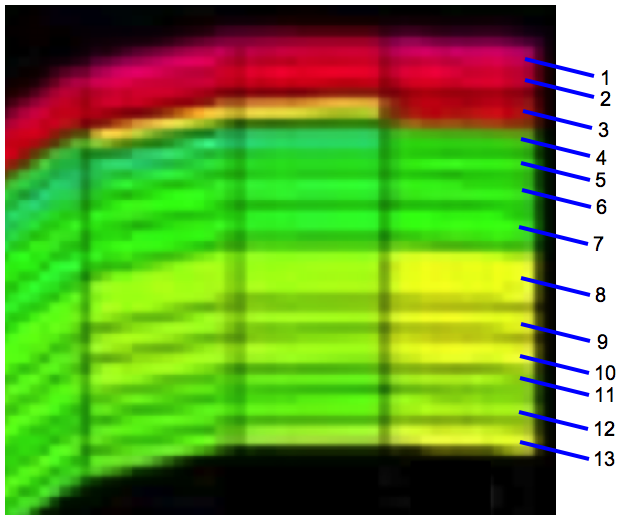
I have numberered the 13 layers that the simulation divides the rock into, and the lateral grid cell index can also be counted off (rather more easily). Once numbered, it is possible to generate a random sample of grid cell addresses, and, using the color scale, measure the saturation in each one. We avoid cells very close to the original oil water contact, and we also avoid cells which have not had the same color for at least a decade (ie where the simulated saturation might still be changing noticeably). In particular, we don't count unswept areas in the final saturation - if any areas are finally unswept we will take account of that in a separate sweep efficiency parameter. This allows us to form a random sample of what the simulator considers the population of block final saturations is, at least for this particular location in the field. Since Saudi Aramco uses state of the art simulation methodologies, has extensive well log data and production history to match to, and since a central point of the simulations is to estimate and maximize ultimate recovery we have reason to think that the simulation's final saturations will have some fidelity to the true situation in the reservoir. The other type of evidence comes from studies of flushing particular samples of rock either in the lab or rock taken from the reservoir after flooding. For example, this next figure shows relative permeability curves for composite samples of rock from three operating areas:
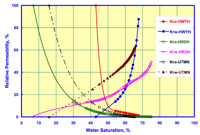
The relative permeability of oil (Kro) represents the ability of that oil to flow as a function of water saturation. When the relative permeability to oil goes to zero (where the oil curves hit the x-axis) then no further oil can flow and the rest will be left behind by the waterflood. As you can see, these particular rock samples had a final water saturation of about 66% in Uthmaniyah, 68% in Hawiyah, and 76% in Haradh. That is to say, that at the end of waterflooding these particular samples, 34%, 32%, and 24% respectively of the pore volume was left with oil that would not come out. Similarly, the initial water saturation represents the point below which water will not flow (ie Krw=0). It is not clear how typical these particular sample are of the areas in question however - there is no reason to expect rock in Hawiyah to be worse on average than rock in Haradh, and we know that in all areas the rock is very diverse and it would be possible to find both good rocks (with a large oil window between the initial and final saturations), and poor rocks with a very small window (such as the Hawiyah sample in the graph above). Hopefully these samples will illustrate the kind of evidence available on saturations; there is too much data to show all of it, but this next figure summarizes the evidence I was able to gather from Saudi Aramco technical papers.
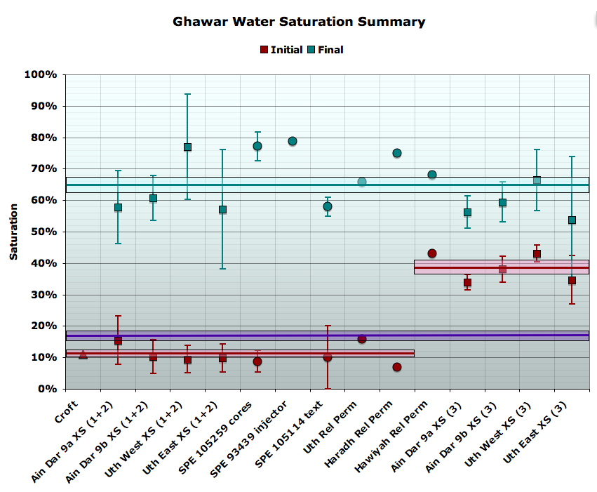
Note that the error bars shown are not the standard error in the mean of each population, but rather the standard deviation of that particular population (whether it be a sample of grid cells in a simulation visualization, or a family of experiments) to better illustrate the variability at a given location, as well as the variability between locations) . As to the final saturations (turquoise data), although there is significant variation from one place to another, there is no obvious trend in the data. Thus, the approach I took was to treat the points on this graph as equally weighted individual observations around the field average for the final saturation. The spread in these observations allows me to constrain an uncertainty for that average. That gives a final water saturation of 65.1% ± 2.4% (percentage point error, not relative error). This is shown as the pale blue box around the 65% point. The only potential problems with this are if either the Saudi Aramco simulations and experiments lack fidelity, or if this sample of observations is somehow too biassed. Overall, there is quite a lot of geographical spread in the field, but it is somewhat weighted towards north Ghawar. So it may not extend quite as well to the south. However, the data points that we do have for the south do not appear at all anomalous relative to the northern observations. The initial saturation data (red) is more interesting and gave rise to an extended debate between Euan and I which ended up delaying this post a week. The first thing to note is that the data appear quite bi-modal. There are a number of observations which cluster around the Croft value of 11% (in fact they average 10.9% with a standard error in that average of only 1.0% (percentage points). There are also a number of much larger values that are closer to 40% (mean of 38.6% ± 2.0%). There are no observations in between. In analyzing the initial saturations in cross sections of simulations I divided the cells into separate observations on zone 2 and zone three, since it was obvious the two were very different. The division between zone 2 and zone 3 is based on layer counting and the following scheme from SPE 84371 (A Scalable Massively Parallel Dual-Porosity Dual-Permeability Simulator for Fractured Reservoirs with Super-K Permeability):
The reservoir model is characterized into four zones. Zone 1 is in layer 1, zone 2 is in layers 2 to 10, zones 3 is in layers 11 to 13, and zones 4 is in layers 14 to 17.If the 'Ain Dar simulation pictures came from a simulation with the same layering scheme, then it suggests that, as there are only 13 layers, zone 4 is not important to production in this area (in general, it is rarely mentioned in the literature). It further suggests the interpretation that the bottom three layers are zone 3. If we now look at an example from 1940, i.e. before production, then we can clearly see the difference in the initial saturation in these layers.

As you can see, the lowest three layers are yellow (40% water) or almost so. The picture in Uthmaniyah is similar. It is plausible that water saturations in the poorer rock of zone three would be higher than in the zone 2 rocks above. However, Euan felt strongly, based on his experience, that 40% water saturation was unrealistic in net rock. He argued that those layers must include rock that would not have been considered net in the Croft numbers, i.e. rock of single milliDarcy permeability or sub milliDarcy permeability. He and I explored data from carbonates in other fields were indeed he would be correct, but didn't find dispositive proof that net pay in Arab-D couldn't have initial saturations that high. Hold that potential issue in the back of your mind for a moment. We have a lot of data on saturations, but we might not know quite how much of the oil they are being applied to. If we average the zone two and zone three values for initial saturation and compute a combined average (using a ratio for net pay based on analysis of the well logs from Powers 1962 paper and simulation cross sections) we get an initial saturation of 16.9% ± 1.2% (percentage points). This gives a saturation change of 48.2% ± 2.6% (percentage points), and a recovery rate of 58% ± 3.2% (before applying any correction for sweep efficiency - blocks that end up unswept). Remember that recovery rate. And remember it just comes from averaging together simulation cross sections and experimental observations that Saudi Aramco has published. Unfortunately, little public data is available to support estimates of sweep efficiency (how much oil that in theory might have been producible but is left behind because the waterflood moves unevenly and leaves some areas unswept). Based on advice from our various pseudonymous and anonymous industry advisers, I adopted an outer range of reasonableness for this well managed waterflood in north Ghawar of 80% to 100%. Thus my central value is 90%, and I take 5% (percentage points) as the 1-sigma error bar. In the south, with poorer rock and heavy fracturing, I used 80% ± 10%. Next, an exercise to validate the original reserve model with the asphaltene map was undertaken. This identified one major area where the linear OOWC model and the broad contour interval combine to miss a low-lying area that is above the oil water contact, and which has a modest number of producing wells in the Voelker well distribution, and industry report maps. Based on estimation of this volume, a 5.5% upward correction was applied to North 'Ain Dar, and 4.5% to Shedgum. No issues were identified in South 'Ain Dar. I compared these estimates with this figure from a 2004 presentation by Baqi and Saleri of Saudi Aramco, endeavoring to refute the concerns of Matt Simmons:

There are a number of very interesting numbers in this graphic. But let's first talk about the recovery rate data. On the one hand for proven reserves we see a claimed recovery rate of 60%, compared to the 58 ± 3.2% we observe by averaging various individual observations in Saudi technical papers. So these numbers are potentially in good agreement (within one sigma) with the exception that proved reserves would be assuming 100% sweep efficiency- a fairly aggressive assumption. More troubling is the estimated ultimate recovery of 75 percent of original oil in place. It does not appear that this ultimate recovery could come from the present peripheral water flood alone. All simulation cross sections in Ain Dar and Shedgum end up at about 65% water saturation - ie 35% of the pore volume is left as oil following the water flood, even in areas that were first swept decades ago. Given that not all the pores began as oil, recovery rates from the flood must be somewhat below 65% under any reasonable assumption. (It's very hard to see how the simulations could be badly wrong on this point, since they would show far more historical production than the actual wells if they were so wrong, making them useless to their owners). If indeed ultimate recovey ends up as high as 75%, it would appear to have to be as a result of extended recovery techniques of some kind, which would of course produce oil at much lower rates. Now let's take our initial and final saturations, together with Croft porosities and pay heights (which recall are circa 1980 Aramco average estimates). I applied those assumptions to the map based model discussed earlier. Doing so resulted in estimates of original reserves for Ain Dar and Shedgum of 28.3 ± 2.1gb, with an estimate for original oil in place of 54 ± 4gb. (The estimate of original reserves for the whole of Ghawar would have been 83 ± 9gb). So there are two discrepancies between the numbers I just mentioned and the Baqi/Saleri slide above. Firstly, they reported cumulative production for this area in 2004 of 26.9gb. If the original producible oil was only 28.3gb, then we'd be left with only a couple of billion barrels by 2004, which would imply the field would have had to be already declining, inconsistent with other data showing it on plateau then. Furthermore, they are reporting far more OOIP - 68.1gb, versus 54 ± 4gb. That's a discrepancy over the central value of more than three standard errors - a pretty material discrepancy. Their value is 25% ± 9% higher. Now, we also have the following graph from the 2004 Aramco presentation concerning the growth of OOIP in the country as a whole:
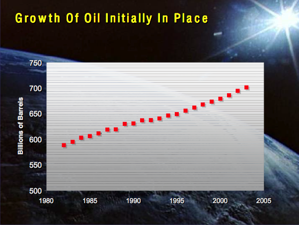
Careful measurement of the first (588.5gb) and last (700gb) data points gives us a whole-country OOIP growth of 19%. So, it would appear the growth in 'Ain Dar at 25% ± 9% is consistent with the whole country OOIP growth. This raises the question of were this extra oil could be? Ain Dar and Shedgum had been in production for three decades by 1980. There would be no potential for growth in the known oil at the edges of the field because the edges of the field had been drowned long ago. In principle, there could have been discovery of additional reservoirs, but this isn't very likely in such an extensively produced and characterized field, and nor is there any discussion in the literature of new reservoirs in Ghawar being studied (though there is ample discussion of deeper Khuff gas reservoirs). This leaves only one real possibility which is that the growth in OOIP is coming from rock that was not previously considered net pay, that is, rock of very low permeability in which oil flows very poorly. Let me at this point remind you of Euan's concern that in the simulation cross sections, the zone three saturations were too high to be net rock. Could there be enough oil in the poor, formerly non-net, rock to account for this OOIP growth? Well, take a look at this next figure:

I have added the blue line as a visual fit to the trend of the data. Our industry advisers, asked about the likely permeability cutoff for net rock suggested values from one milliDarcy to 10 milliDarcy circa 1980. In my log analysis I used three milliDarcies. As you can see, in the plot above, these cutoffs would leave rock with a significant amount of pore space and a sizable fraction of the rock would be below these cutoffs. for example, the 3 milliDarcy line hits the trend at 14 percent porosity. Overall, this suggests that including all of gross rock in OOIP could lead to about the right amount of growth, though it's hard to be certain based on one well. At any rate, the stance taken here is that we should give Saudi Aramco the benefit of the doubt wherever there is any, and see if we have established a problem notwithstanding that. Thus, I assume that the saturation figures derived above (from Saudi Aramco simulations and experiments) should be applied to the "grown" OOIP that they say they use, and I use the 700/588.5 change as a basis to estimate that growth factor. As we will see in the sequel, once this is done then all evidence forms a consistent picture of the state of the field. To begin with, we can examine the implications of the 26.9 gigabarrels of cumulative production to date. Because my model allows me to estimate the volume of rock in the field I can infer how high up the structure the oil water contact must have risen in order to produce 26.9 gigabarrels of oil. It turns out a 511 foot rise is the number required, which can be the basis for comparison with other estimates of the OWC height. Let us take one more step before we do that. We know the production history in North Ain Dar through 2004 from Figure 1 of SPE 93439 (the North 'Ain Dar water management paper):

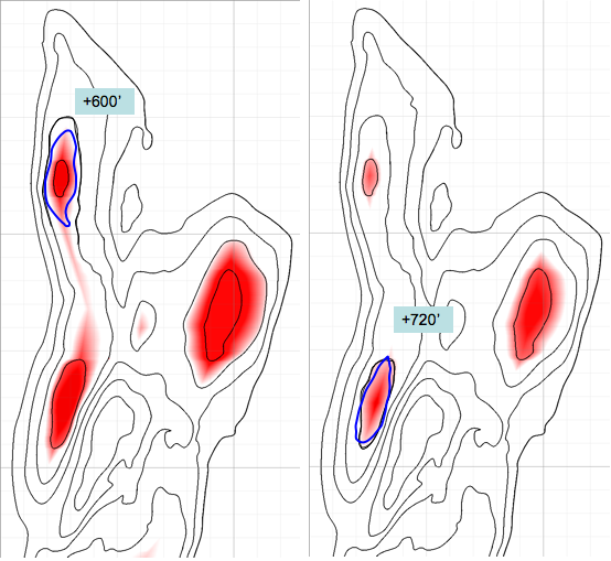
With my 3D model and the above assumptions about saturations, etc, I can figure out how much change in the average OWC in North Ain Dar is required for each unit of production. So I can take the 511' offset in OWC inferred from the entire Ain Dar/Shedgum cumulative production by 2004, and then back it down the North Ain Dar structure to give the right production history for that subregion. If I then plot that with all the other data we have on OWCs in this region, it looks like this:

In addition to the data described earlier, I have added the gas cap base (treated as though it was at the top of the structure, which it isn't actually), and the OWC curve inferred from reversing production as just described. The level of agreement on the state of the field circa 2004, and over the last 15 years or so, strikes me as extraordinary. Given the diversity of approaches summarized in this graph, it seems very unlikely that the conclusions about current OWC could be badly wrong. Unless the gas cap model is systematically wrong, it's hard to see how production in North 'Ain Dar could not be affected by now. The production based OWC estimate was divergent from the linear 18.4 foot/year vertical rise line prior to the late 1980s, and follows a more physically realistic track for average OWC. My interpretation of what happened is that during the 1960s and 1970s, under heavy production, water crossing the broad very shallowly angled plateau northeast of the north 'Ain Dar crest was in poorer gravitational compliance, with oil piled up before the advancing water, and water not penetrating the less permeable lower strata of the reservoir as fast as static gravitational equilibrium would have dictated. Thus the ridge areas studied in SPE 93439 did not get water until a relatively late date in the second half of the 1970s. However, in the 1980s, as the OWC got into areas where the structure is steeper, and as production was sharply reduced due to the demand destruction following the 1979-1980 oil shocks, gravitational compliance improved and the OWC in the north ridge area began to track the average OWC based on production quite well. From the 511' offset, I can plot what the distribution of remaining oil would look like. (Note that this is just moving the original OWC plane up 511' without changing its tilt in any way - this is not likely exactly what happened, but is as good an assumption as any, and the Linux supercluster picture suggests it is not very wrong) Here is a comparison of the original and remaining reserve distribution under that assumption:
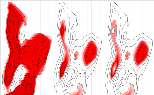
For comparison, here is the Linux supercluster picture again. Clearly, the Linux picture is either not simulating the gas caps, or is actually plotting "hydrocarbon saturation" 
To my eye, this picture is generally compatible in showing oil mainly up in the crests, roughly in compliance with gravity, though with some deviations where the supercluster picture has more oil in the saddles between the crests, while my model has a little more on the crests. However, it is hard to make a more precise comparison than given above, given the different view angle and the small scale of the Linux picture. This concludes the detailed analysis of the 'Ain Dar/Shedgum regions. I now turn to the simpler treatments I used in the other regions.
UthmaniyahOriginal reserve analysis in Uthmaniyah is based on the Croft map and the global OOWC plane for the whole field, Croft table parameters, the same saturation end points and OOIP growth as in 'Ain Dar/Shedgum, and a 20% map correction as discussed above.2004 reserve analysis in Uthmaniyah is based on visual estimation of the full-oil-layer equivalent area implied by three sources: the Linux supercluster visual, 2004 simulation cross sections from SPE 98847 (the water management in Uthmaniyah paper), and a partial map of the thickness of the oil layer from here.
Based on visual examination of the cross sections, it seems clear that with the dual crest structure in Uthmaniyah almost all the remaining oil is in the saddle between the two crests, and the approach based on gravitational compliance, which worked so well in 'Ain Dar and Shedgum, would fail here. Thus 2004 reserve estimates in Uthmaniyah were based on the area analysis above, Croft table parameters, the same saturation end points and OOIP growth as in 'Ain Dar/Shedgum, and a 20% map correction as discussed above.
Southern GhawarLess effort was made to characterize Southern Ghawar as precisely as the north. In general, it is clear that the southern regions will be on plateau for decades at current production rates, and are unlikely to be an important factor in recent Saudi production declines.Original reserves were based on Croft map parameters, the global OOWC map (with correction for tilt in Haradh as discussed above), and a slightly lower 80% sweep efficiency. 2004 reserves were based on the above, plus visual estimation from the Linux supercluster map that oil was 1/8 of the way up the structure in Haradh, and 4/15 of the way up in Hawiyah.
Summary of Uncertainty AnalysisIn this section, I summarize all the various strands of uncertainty reasoning discussed above, and combine them into my current quoted error bars.The overall reserve estimates are of the form of a product of six factors:
Uncertainties in Original Reserves
Uncertainties in Current Reserves
The relative uncertainties are largest in 'Ain Dar/Shedgum in 2004, especially North 'Ain Dar. The reason for this is that there is not much oil left there, so small changes in the position of the OWC make large proportional differences in the estimated reserve remaining. Comparison with Euan MearnsThe other week, Euan Mearns presented his latest thoughts on the status of Ghawar, and its production prognosis. In this section, I compare my subfield estimates to Euan's. Note that Euan's estimates were revised based in part on seeing some of the reasoning behind this post (particularly the 'Ain Dar saddle decode). The largest remaining points of difference in how I estimated original and remaining reserves versus Euan are:
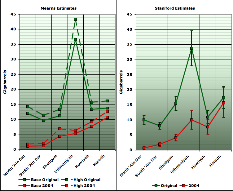
Overall, you can see that our estimates are in fairly good agreement. One of the wonderful properties of independent errors is that they tend to cancel to a significant degree, and here we see the varying effects of our different procedures mostly canceling. Here is a more direct comparison of our estimated ultimate recovery estimates:
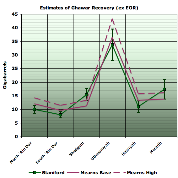
Whole Field ComparisonsBoth Euan's and my estimates can be compared to that of others on a whole-Ghawar basis. For comparisons of Ghawar as a whole, the following figure gives estimates by a variety of organizations of original reserves and remaining reserves. Where necessary, I have adjusted from the estimate date to a common 2004 date by adding or subtracting production in intervening years.

Implications for ProductionIn my view, the best way to assess the implications of the depletion status of north Ghawar as shown in this analysis is to look at the reserve/production ratio. If we assume that declines are uniform after a field goes off plateau, then there is a mathematical relationship between the final R/P at the end of plateau and the decline rate. In essence, the closer to empty an operator can keep the field on plateau, the worse the decline will be when it comes:

In the 1979 Senate report, it was anticipated that Ghawar declines would begin between 1993 and 1995, based on being unable to maintain plateau once R/P was less than 15 or 20 (corresponding to a post-plateau decline rate of 5%-6%). This was based on all vertical wells. Modern technology has allowed maintenance of plateau to R/Ps below 10, and perhaps even below 5 in some cases. This gives rise to very aggressive declines of 10% or 15% or so respectively once plateau is lost. This next graph gives my estimates of R/P for the Ghawar operating areas. The assumptions made here are that the split between South 'Ain Dar and Shedgum of the 1.5mbpd they are known to share on plateau is 0.5mbd to South 'Ain Dar, and 1mbd to Shedgum. Also, North Uthmaniyah's plateau is assumed to still be the 1.9mbpd documented in the 1979 Senate report. Either or both of these assumptions could be slightly off.
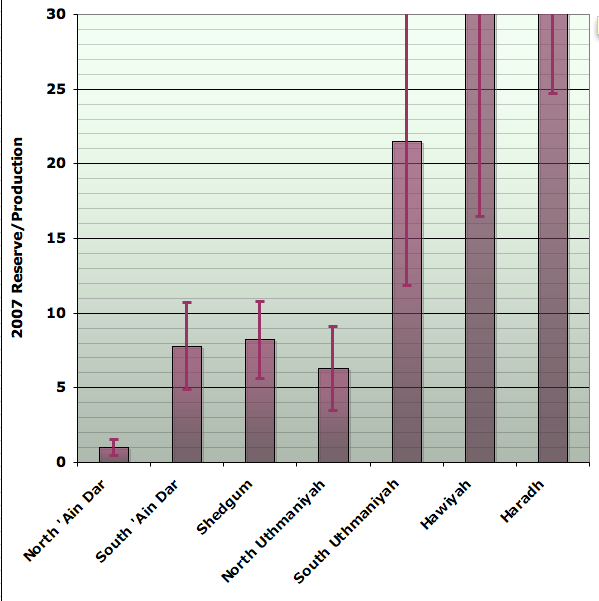
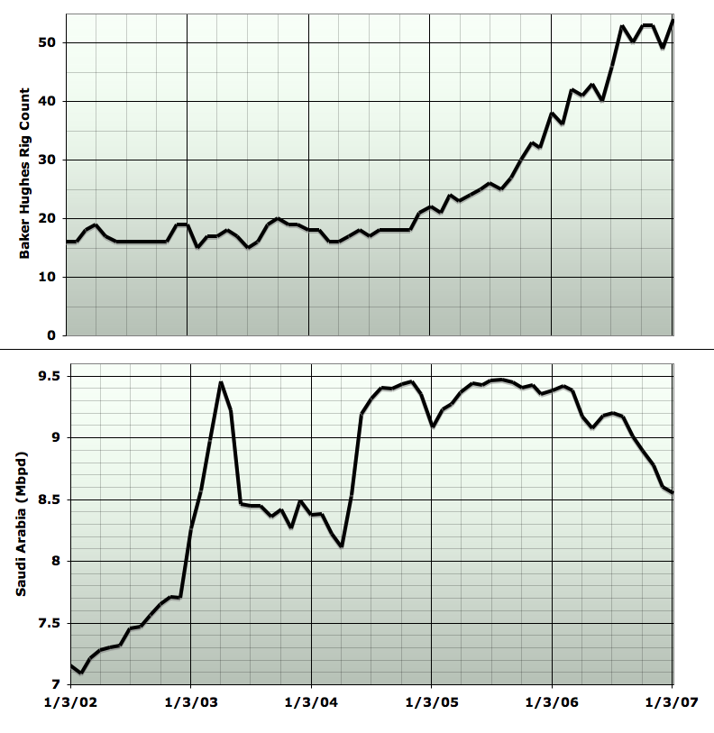
As you can see, the whole of North Ghawar is either off plateau already, or getting close. That is something like 3.9mbpd of production based on last known figures. Whatever of this decline has not already occurred will mostly occur during the next decade. Southern Ghawar, by contrast, can maintain plateau for decades to come, but there is only 1.7mbpd of production there on last known figures. While we cannot attribute an exact fraction at this time, it seems likely that not-altogether successful attempts to maintain the north Ghawar plateau to the bitter end explain a significant fraction of the sharp increase in oil rigs that began in 2004, as well as the production declines since that timeframe:
AcknowledgementsIt is a great pleasure to acknowledge the enormously fruitful collaboration I have had with Euan Mearns on this issue, as well as with Fractional_Flow. We have exchanged literally dozens of emails a day for months. Euan's deep and original thought, and his insistence on my proving every point of my contentions has immeasurably improved the product - indeed the project likely would not have existed had Euan not challenged my views. Fractional_Flow led us into the Saudi petroleum engineering literature and has been a consistent source of provocative new ideas, professional experience, and references.Additionally, a now sizeable group of oil industry professionals have reviewed parts of this material, helped us understand and debate the issues, and provided key references. Several have contributed quite large amounts of effort to assisting us. They prefer to maintain their anonymity, but their contributions are greatly appreciated. Finally, numerous commenters at The Oil Drum have contributed critical references, ideas, and valuable critiques over the last two months. Their contributions have been essential. Notwithstanding, this piece expresses my views alone. Please bring any errors to my attention and I will attempt to fix them.
Stuart Staniford has a PhD in Physics, MS CS. 10 years as an innovator in computer security (especially worms). Patents, research papers with 100+ citations, major media coverage. Ran a company for 5 years. Now working as a consulting scientist and researching peak oil. |
| Home :: Archives :: Contact |
TUESDAY EDITION July 14th, 2026 © 2026 321energy.com |
|